How To Merge Duplicate Rows or Cells In Google Sheets-6 Way

Merging duplicate rows is considered an elaborate task that often discourages users due to its complex functions and formulas used in achieving this feature. Merging rows primarily depends on the cells in the main column and other columns in the worksheet.

One must understand the differences between merging and removing duplicate rows to make tasks performed with this feature as easy as pie.

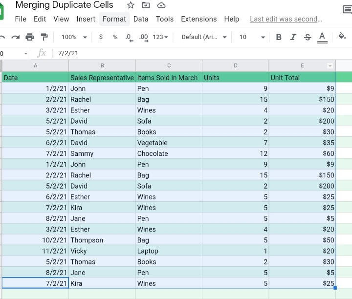
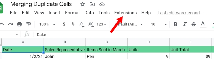
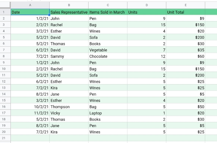
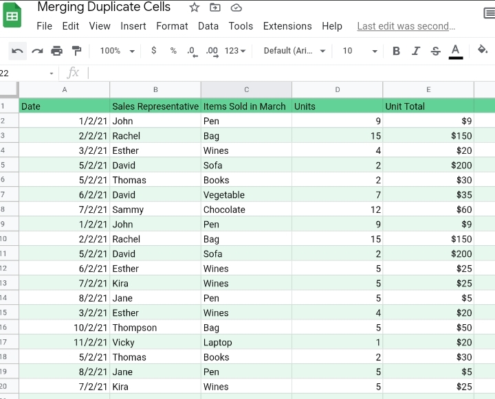
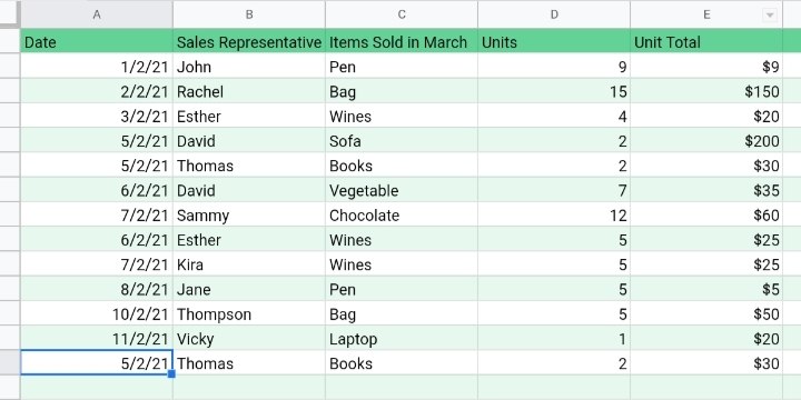
In this tutorial, we will discuss the six basic methods used for merging duplicate and repeated rows in Google sheets with references to the sample worksheet below.

Method 1: The Concatenate Values to Merge Duplicates Rows in Google Sheets.

The Concatenate function is a tool used for removing and combining duplicate rows. First and foremost, you would have to organize your dataset accordingly. You can merge cells in Google Sheets with the formula below.

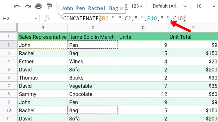
=CONCATENATE “(dupli1, ” “, dupli2, ” “, dupli3, ” “, dupli4)”

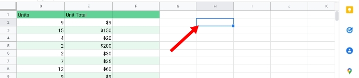
Step 1: Select a row in a separate column from the main data set.

Step 2: Input the above formula in H2 where the duplicates cell references are inputted in the formula.

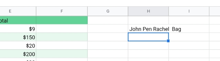
Step 3: Click Enter. The duplicate cells are to form one single string of words.

Step 4: Select the cell reference of the new data.

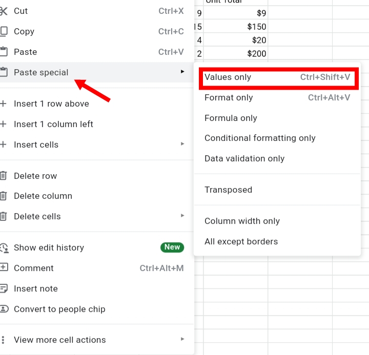
Step 5: Right-click on the mouse. A list of options is provided as seen below.

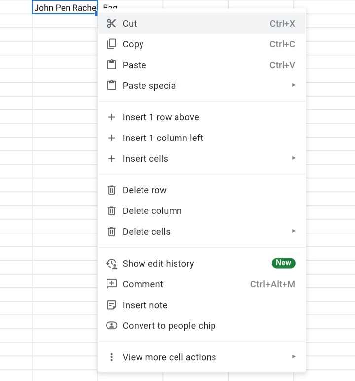
Step 6: Click on Paste Special.

Step 7: Select Paste Values Only. This removes the formula and pastes only the values on the worksheet.

This method is used for small sets of data where you can easily see and point out the duplicates easily to the formula. This does not apply to large data sets. For large data set you follow a further method.

Method 2: Keeping Data with UNIQUE+JOIN Function to Merge Duplicate Rows in Google Sheets.

This method locates and merges repeated data using the UNIQUE and JOIN functions in Google Sheets. It also combines rows based on the duplicates. 

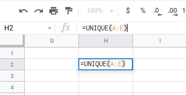
It requires the UNIQUE function to identify the duplicates using the formula =UNIQUE(cell range). This formula generates a list of all dates, names and units sold with or without duplicates as a whole.

[=UNIQUE(A:E)]. This permits editing and the addition of new data to the selected range.

Step 1: Select the range of cells containing the duplicate cells.

Step 2: Input the formula =UNIQUE(A:E) into an empty cell H2, on the right side of the worksheet. This allows easy comparisons between the original worksheet and the results produced.

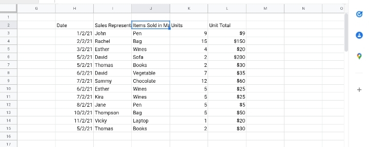
Step 3: Click Enter. The duplicate rows are merged.

Step 4: Select the entire range of the new data.

Step 5: Right-click on the mouse. A list of options is provided as seen below.

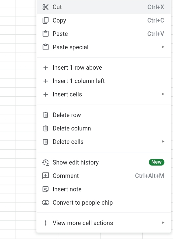
Step 6: Click on Paste Special.

Step 7: Select Paste Values Only. This removes the formula and pastes only the values on the worksheet.

For the JOIN function, the formula is a combination formula consisting of JOIN and FILTER functions which take the format below.

=JOIN(“, “, FILTER(column2:column2, column1:column1 = cell reference)

Where;

1. FILTER function scans column 1 for all replicas of value and displays them in the cell reference. It extracts corresponding data duplicates from column 2.
2. JOIN function unites these values in a single cell with a comma.
3. Column1 represents Column A.
4. Column2 represents Column B.
5. Cell reference refers to the row which you want to merge the cells into.

With the following steps below, we would show you how to merge cells using the JOIN function.

Step 1: Select an empty row as the cell reference where you input the formula.

Step 2: Input the formula =JOIN(“, “, FILTER(B:B, A:A =H2) in H2 as the cell reference.

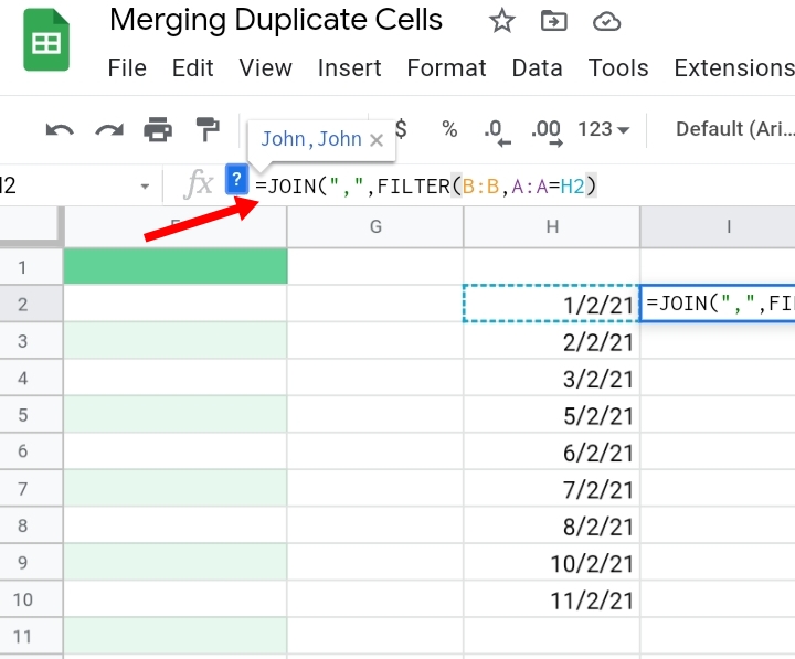
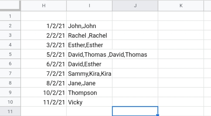
Step 3: Click Enter on your keyboard and the extra data copies are merged in one cell each.

Method 3: The Query Function to Remove Duplicate Rows in Google Sheets.

This is another technique used for removing duplicates. The query function selects certain columns in your worksheet and deletes duplicates from them. 

Due to its broad range of commands, the QUERY function is considered a tricky and difficult function for beginners. Here, we would simplify the query function best to your understanding.

The query function is stated as seen below.

=QUERY(data, query,[headers])

Where;

1. Data represents the range of cells.
2. Query represents a set of commands used to determine conditions to get specific data.
3. Headers are the number of header rows in your worksheet. It is not a compulsory component of the formula.

The query function operates on a given set of conditions on what values you want to extract from your worksheet. The given commands are:

1. The SELECT command to choose the cell you want to query.
2. The GROUP BY command to group the values across the selected cell range. The Group by command works when you apply one of the statistical functions (avg, max, sum, min) etc, within the select command.
3. The WHERE or OFFSET command omits an empty row in the worksheet.

These commands take the following order

“Select A, sum(B), C, D group by A, C, D offset 1″

Therefore, the formula is written like this.

=QUERY(A2:E, “select A, sum(B), C, D, group by A, C, D offset 1”)

Where;

• Select A, sum(B), C, D- the selected columns.
• Sum(B)- we have to apply a statistical function in the select command so we chose Sum.
• Group by A, C, D-  the selected column to group by.
• Offset 1- used to delete the blank row at the top of the worksheet.

The query function is not the best way to merge cells but it does serve its purpose in Google sheets.

Method 4: The Use of Power Tools.

Power tools are added features and tools that can be installed from the Google Marketplace to your worksheet. 

These tools are a collection of add-ons that boast as important time-savers when working with large data on a Google sheet. These power tools are easy and help to

●      Organize your formulas in one place.

●      Merge Rows.

●      Remove duplicates in cells.

●      Functions are stated in one place.

●      List unique values in your data and many more.

If you don’t have this Power tool and you want to install this feature to your Google sheet, you should follow the steps listed below.

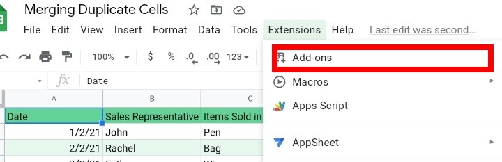
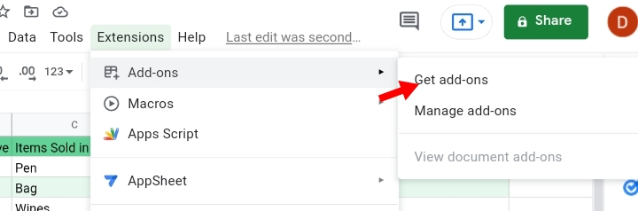
Step 1: Click on Extensions on the toolbar.

Step 2: Click on Add-Ons.

Step 3: Click on Get Add-ons.

Step 4: You would be redirected to the Google Workspace Marketplace website. Various apps, innovations and tools are sold here. Some are paid for while some are for free.

Step 5: Search for Power tools in the search bar.

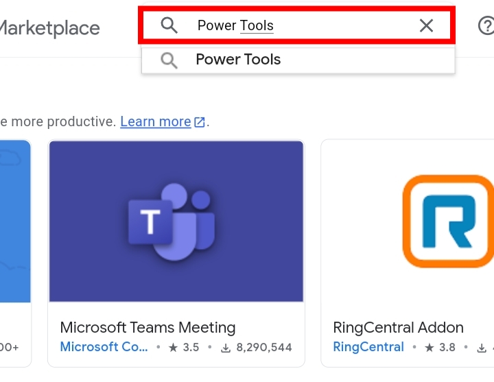
Step 6: The Power tool feature is displayed on the screen.

Step 7: Click on the app. Click on Install.

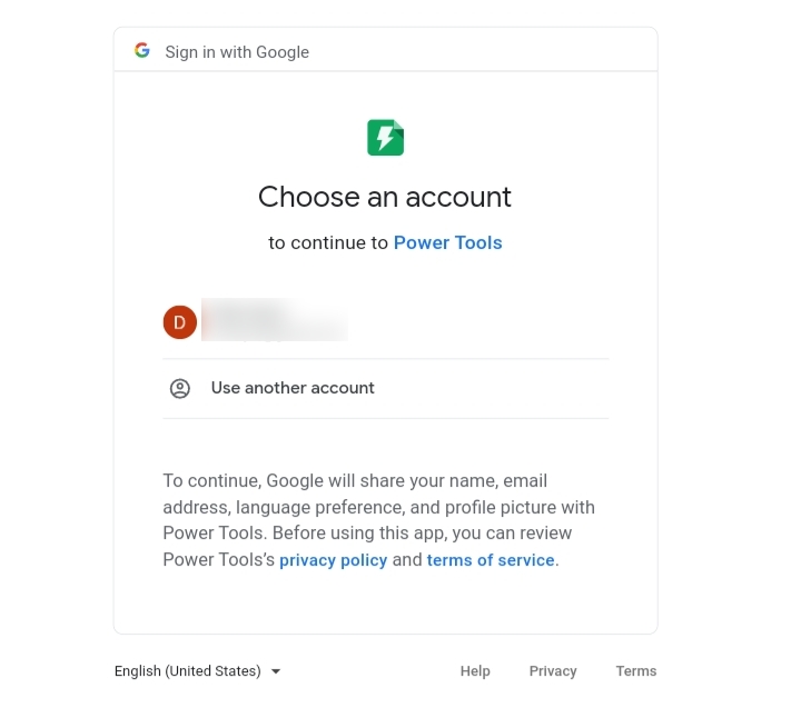
Step 8: You have to grant permission for the power tool to access your Google sheet.

Step 9: You would be redirected to confirm your google account to be linked with the power tool.

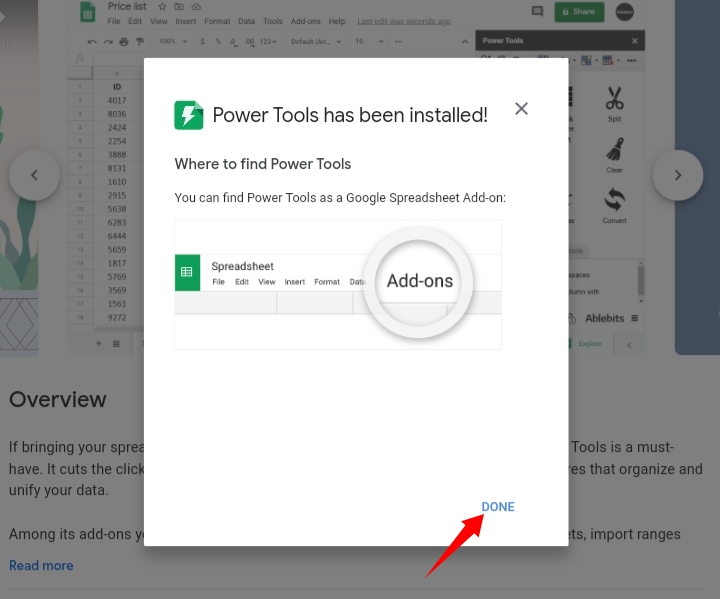
After the permissions are granted and the account has been verified, the power tool becomes installed as an add-on in your Google sheet.

Click on the Done for successful install.

Step 10: The power tool is categorized under the Add-ons tab.

This power tool is the easiest and most effective method for combining cells using the listed steps below.

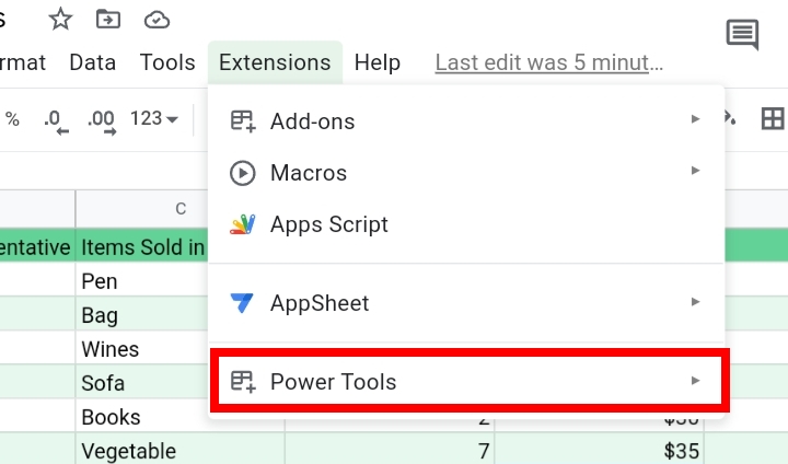
Step 1: Click on Extensions on the toolbar.

Step 2: Select Power Tools.

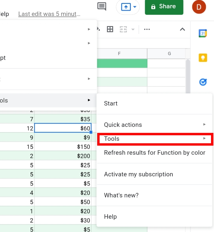
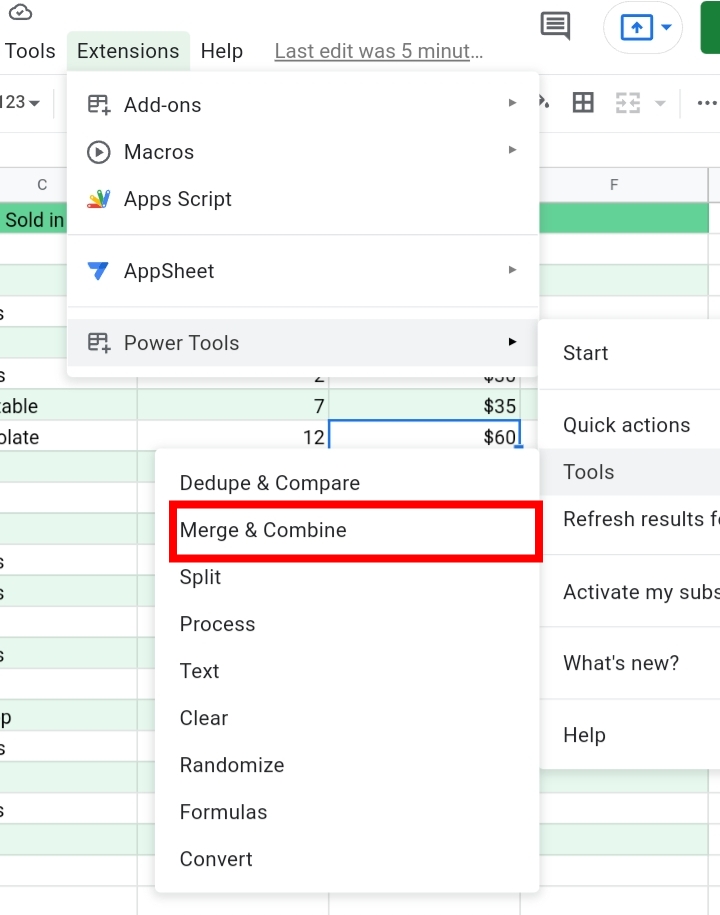
Step 3: Select Tools.

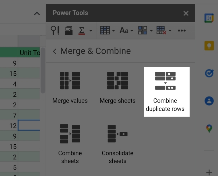
Step 4: Click on the Merge and Combine tool.

Step 5: A new tab appears on the right side of the worksheet. Select Combine duplicate rows.

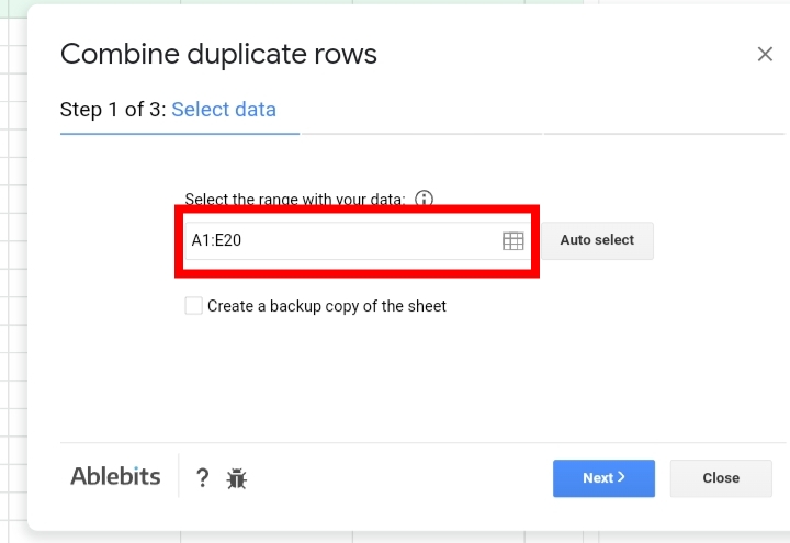
Step 6: Select the range of data.

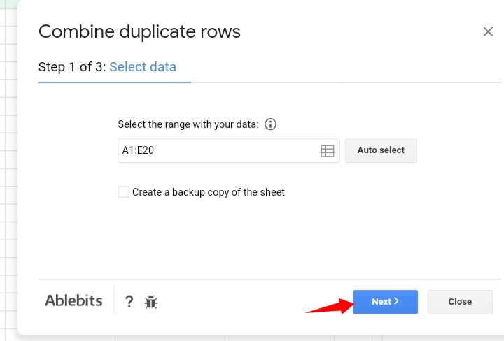
Step 7: Click Next.

Step 8: Next, you choose the columns with the values you want to merge.

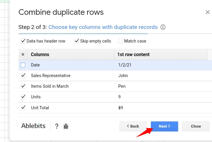
Step 9: Select the column header, the delimiter that separates and differentiates the duplicates and the calculation of the values if the worksheet has numerical data that you want to perform statistical functions on.

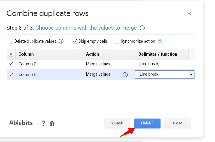
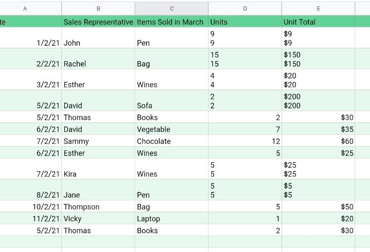
Step 10: Click Finish. The results of the merging.

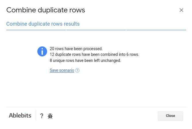
All duplicate data and cells are successfully combined to aid understanding.

Method 5: Merging and Unmerging Cells using the Format tool.

This is also an easy method used to merge and unmerge duplicates in Google sheets.

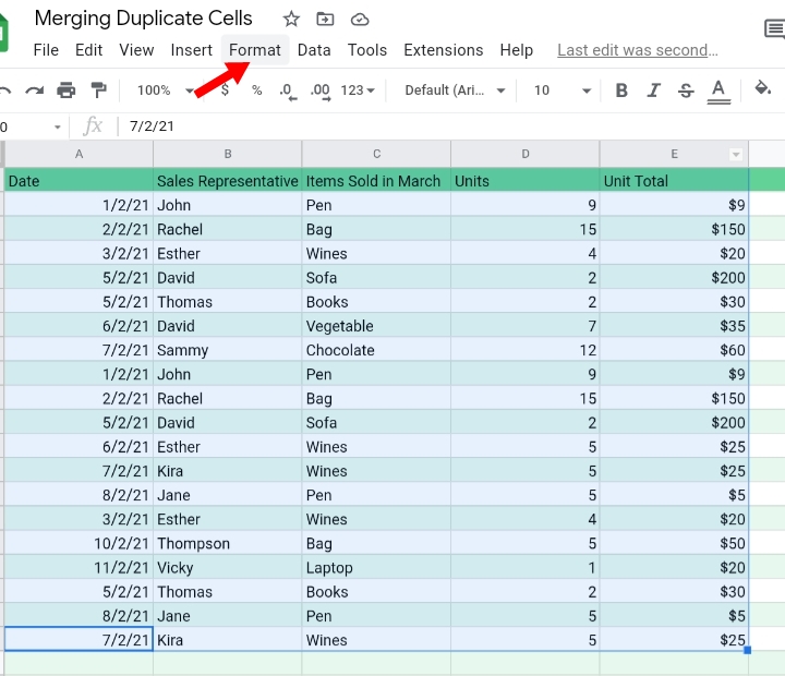
Step 1: Select the data range.

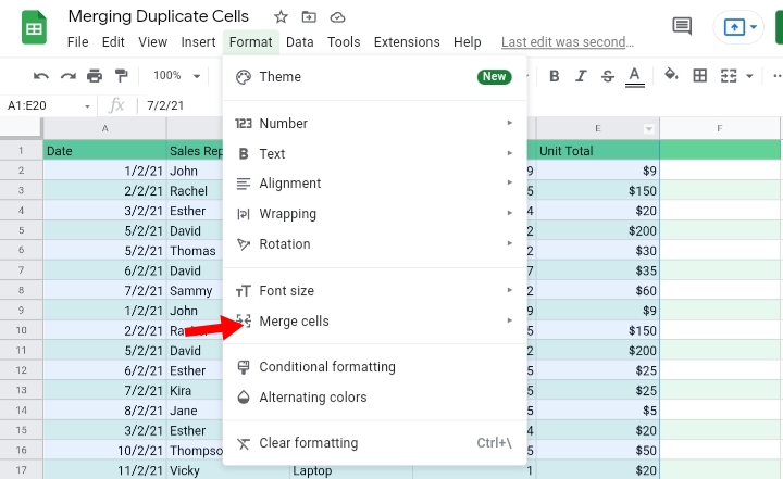
Step 2: Click the Format feature on the toolbar.

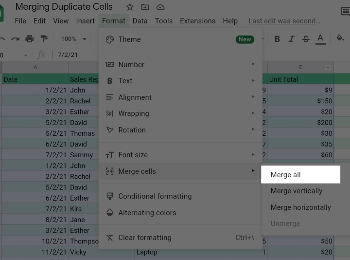
Step 3: Click on Merge Cells.

Step 4: Select Merge All.

Step 5: A warning pop-up is displayed on the window stating that only the top leftmost value would be retained.

Step 6: The top left value is retained, and all other values are merged into a big block.

Note: Duplicate cells can also be merged in horizontal and vertical order.

If you want to unmerge the merged cells,

Step 1: Select the merged data range.

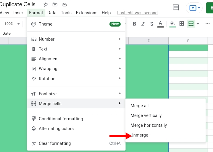
Step 2: Click the Format feature on the toolbar.

Step 3: Click on Merge Cells.

Step 4: Select Unmerge.

Step 5: The merged rows are returned to their original version.

Method 6: Removing Duplicates with the Data Tool.

Also, another technique used for removing duplicate cells is the use of the Data feature on the toolbar.

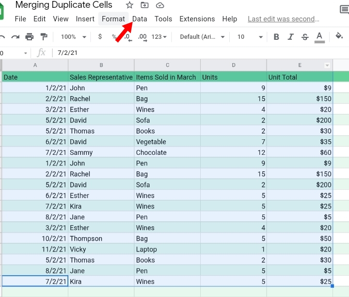
Step 1: Select the data containing the duplicates.

Step 2: Click on Data on the toolbar.

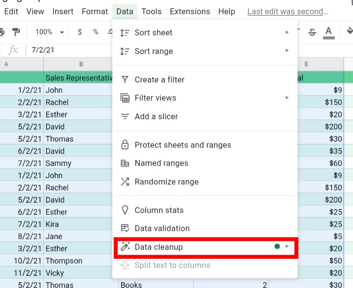
Step 3: Select Data Cleanup.

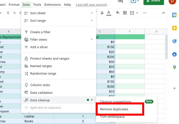
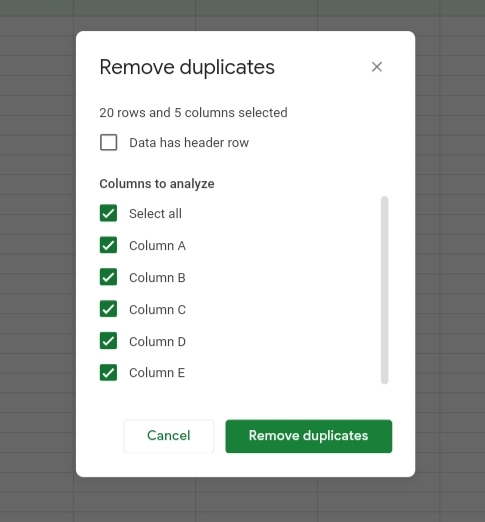
Step 4: Select Remove Duplicates.

Step 5: A list of options is provided on what you want to remove. Select everything on the list depending on what you want to remove. Note that you can check against any column in your worksheet.

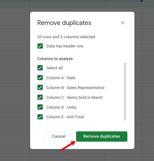
Step 6: Select Data has header row and click on Remove Duplicates.

Click on ok option.

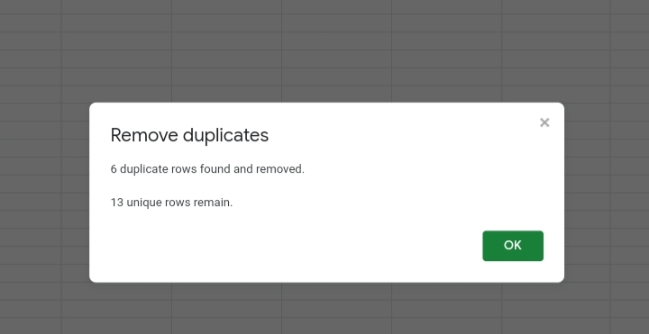
Step 7: All duplicates in the worksheet are removed.

Final Thoughts:

With the detailed steps explained above, merging and deleting duplicate cells is made understandable for Google sheets users. I hope you found this guide worthwhile. Thank you.