Google Sheets provides you tools that can do simple tasks like making a chart, graph or a simple mathematical formula, or can do more complex tasks like making a loan amortization schedule in a very simple way, thanks to the built-in financial functions.
A loan amortization schedule is a very powerful tool that can help you see how your monthly payments affect the overall cost of your loan.
In this tutorial, we’ll learn how to make a loan amortization schedule from A to Z.
What is a Loan amortization schedule?
An amortized loan is one in which the borrower is required to make periodic, scheduled payments that are applied to both the principal and interest.
An amortized loan payment pays off the interest expense for the period first, then applies any remaining funds to the principal balance.
So, we can now say that Loan amortization is the process of scheduling a fixed-rate loan into equal payments, where the interest portion of each instalment is deducted, and the remainder is applied to the loan principal.
Amortized loans can be Auto loans, student loans, home equity loans, personal loans and fixed-rate mortgages.
Amortization tables are helpful since they show you how your debt will be paid off.
An amortization schedule will show you how much of each monthly loan payment is used to pay the principal and how much is used to pay the interest over time.
How to create a Loan amortization schedule in Google Sheets?
We can use the powerful financial functions provided by Google Sheets to create a loan amortization schedule, whether the periodic payments are on a weekly, fortnightly, quarterly, or monthly basis, we would use the same formulas.
In this example, we’ll create a loan amortization schedule based on a monthly periodic payment.
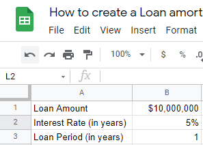
1. Write the input values in the loan amortization schedule.
2. Prepare the format of the loan amortization schedule:
Make 5 column tables to write the formulas in.
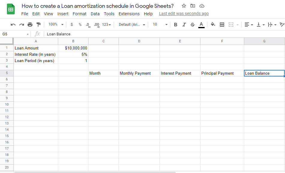
Now, we need to fill the loan amortization schedule using the below formulas.
Check out How To Calculate P-Value In Google Sheets.
Formulas to Create an Amortization Schedule in Google Sheets.
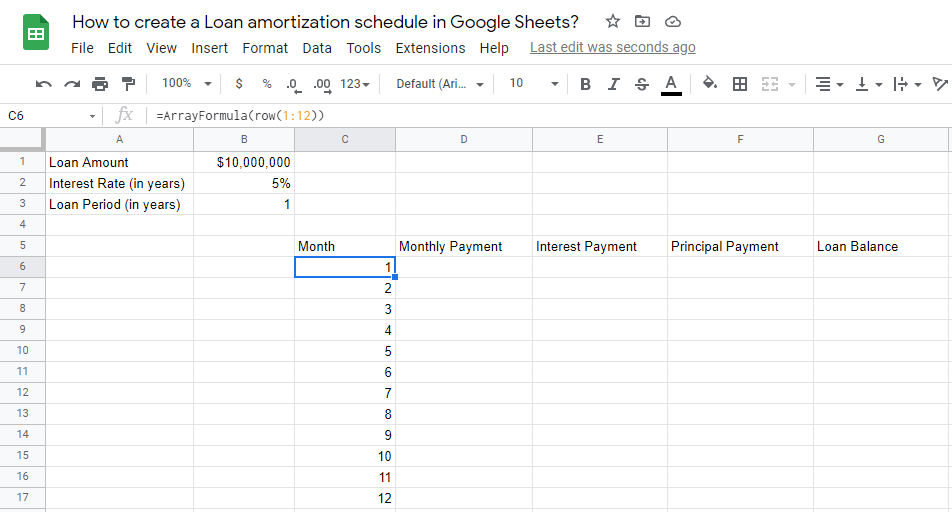
1. Month:
In our example, the loan period is 1 year, which means we have 12 months.
To write it in the form of a formula, we’ll write in the first cell of the months: =ArrayFormula(row(1:12))
2. Monthly Payment:
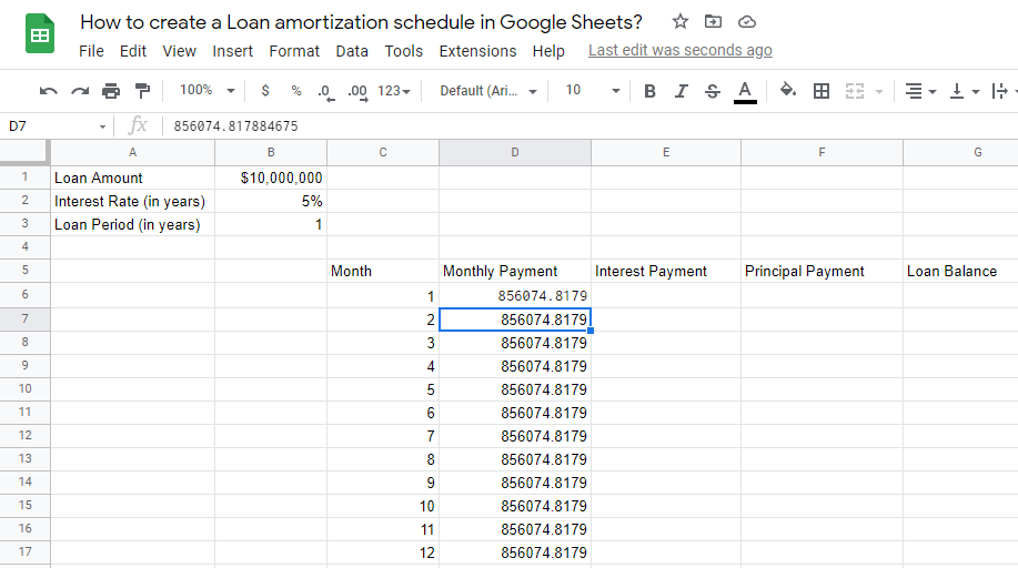
In order to calculate the monthly payments, we’ll use the PMT function.
=PMT(rate, number_of_periods, present_value)
- rate: the interest rate.
- number_of_periods: the number of payments to be made.
- present_value: this will be the principal amount.
So, our formula will be:
=PMT($B$2/12,$B$3*12,$B$1)
To make it easier for you to add the formula in the spreadsheet, we made a
=ArrayFormula(if(len(C6:C),-pmt($B$2/12,$B$3*12,$B$1),))
Notes:
- You can use the non-array formula, but it will give you a negative value, which indicates an outgoing payment.
- All the cell references are locked using the dollar sign ($) symbol because the reference to the cell does not change as our rows change. We want to make sure we are taking from the same values every time.
- Our interest rate is divided by 12 because there are 12 months in a year.
- Our number of periods is multiplied by 12 because there are 12 months in a year.
3. Interest payment:
We’ll use the IPMT function to get the interest payment.
IPMT(rate, period, number_of_periods, present_value, [future_value, end_or_beginning])
- rate: the interest rate.
- period: loan amortization period.
- number_of_periods: the number of payment instalments.
- present_value: this will be the principal amount.
- future_value (optional). It is the future value remaining after the final payment has been made.
- end_or_beginning (optional). It specifies if the payments are at the end (0) or start (0) of each period. By default, this value is 0.
So, our formula will be:
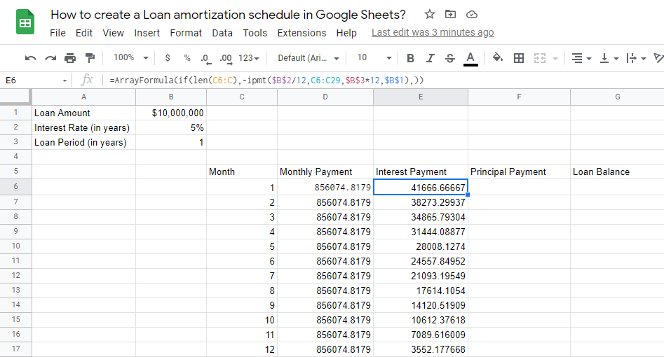
=-ipmt($B$2/12,C6,$B$3*12,$B$1)
You can also use the array formula:
=ArrayFormula(if(len(C6:C),-ipmt($B$2/12,C6:C29,$B$3*12,$B$1),))
Note: We didn’t lock the period reference with the dollar sign ($) because this value needs to change with every row.
4. Principal payment:
There are many ways to calculate the principal payment:
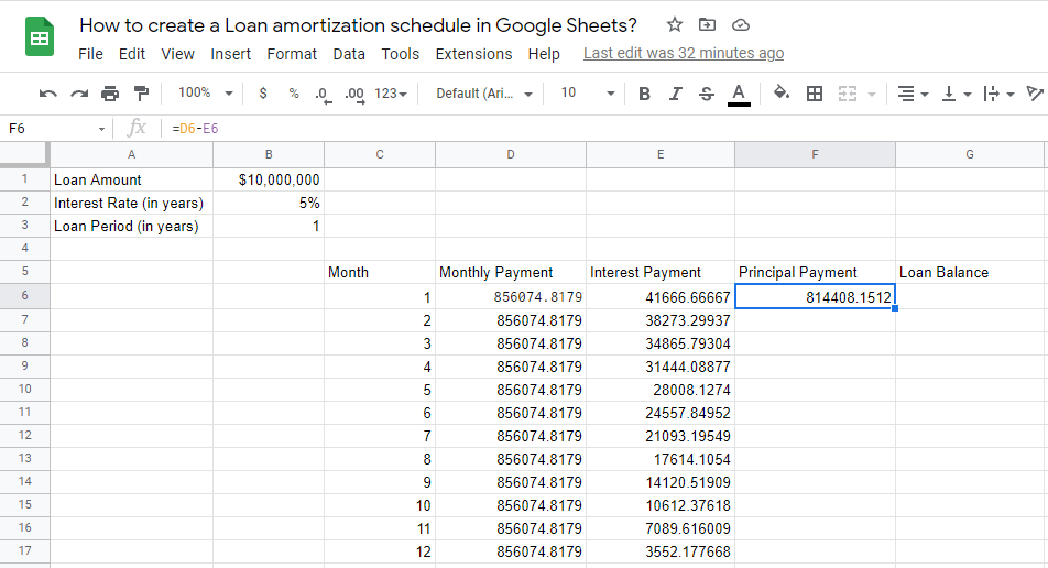
- Principal payment = (Monthly Payment – Interest Payment)
Where the first row equals zero because there is no payment being made. =D6-E6
- Using the PPMT function.
=-ppmt($B$2/12,C6,$B$3*12,$B$1)
- Using the array formula.
=ArrayFormula(if(len(C6:C),-ppmt($B$2/12,C6:C29,$B$3*12,$B$1),))
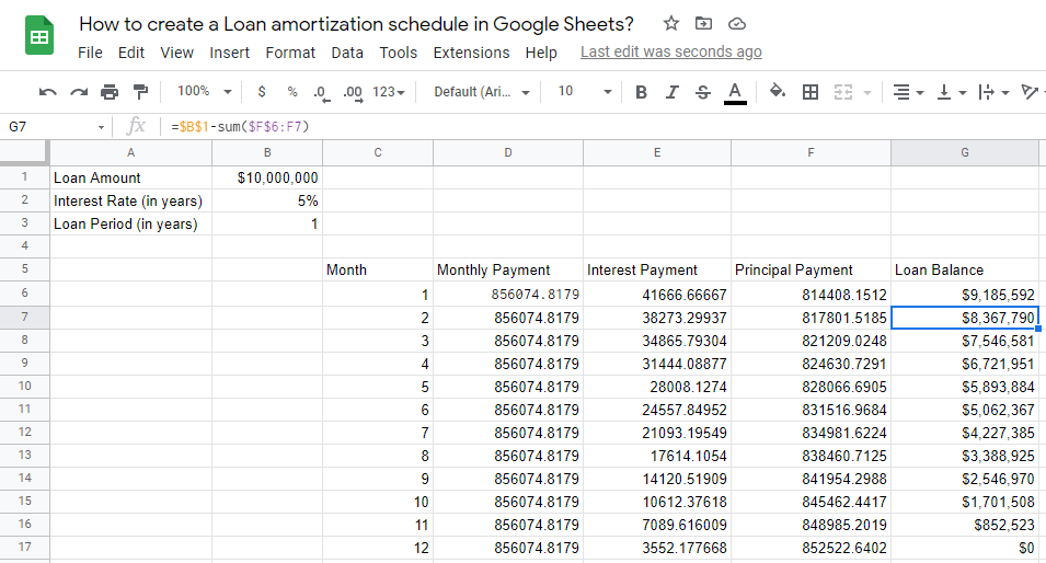
5. Loan Balance:
Write down the following formula:
=$B$1-sum($F$6:F6)
Check out How To Find Slope On Google Sheets.
Change Amortization Schedule Payment to Weekly, Fortnightly, or Quarterly Basis.
Now, we have created a loan amortization schedule, lets change the scheduled payments to weekly, fortnightly or quarterly basis.
You can simply do it by changing them in the previous formulas as explained.
- Weekly Interest Rate = Yearly Interest Rate / 52
- Weekly loan period = Yearly loan period * 52
- Fortnightly Interest Rate = Yearly Interest Rate / 26
- Fortnightly loan period = Yearly loan period * 26
- Monthly Interest Rate = Yearly Interest Rate / 12 (As seen in our example)
- Monthly loan period = Yearly loan period * 12 (As seen in our example)
- Quarterly Interest Rate = Yearly Interest Rate / 4
- Quarterly loan period = Yearly loan period * 4
How to create an Amortization Schedule With Extra Principal Payments in Google Sheets?
Except for the PMT, none of the Google Sheets built-in capabilities will enable you to make extra payments. Here, we need to take a different strategy. That is also not overly difficult.
We’ll be changing our example and add a new column to show your extra principal payments in each quarter this time.
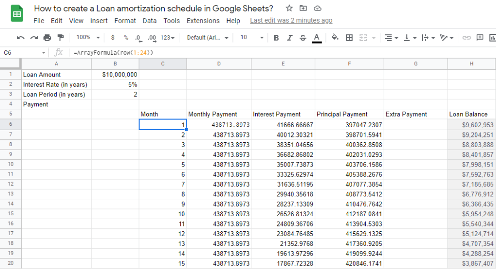
Numbers series in the Range C6:C29:
In the given range, enter the numbers 1 to 17. This time, we’ll not be using the row formula.
There are actually 24 months and the payment is made on a monthly basis. So, why are we having a period of 17 months not 24 months?
Every month, I’m going to make an extra principal payment of $500.00. As a result, at the end of the 17th month, the future value (FV) will be 0.
In B4, use the PMT Formula to calculate the periodic payment:
Instead of using the PMT formula in D6, I’m using it in cell B5. We’ll achieve the same result in B5, but we’ll have to include a logical IF statement there.
To begin, type this formula into D6.
=-pmt(B2/12,B3*12,B1)
Get the Loan Amount, by typing this formula in H6.
=B1
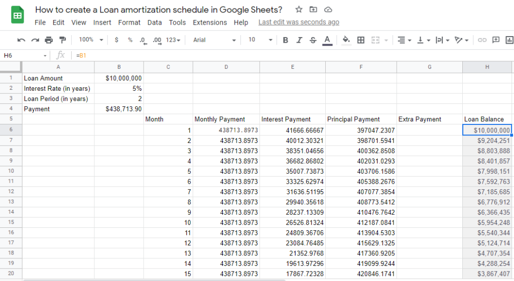
PMT and IF Logical:
Use this calculation in D6 to obtain the PMT value from B4.
=IF($B$5<=G9,$B$5,G9+(G9*$B$2/12))
The loan balance column H in the row above is checked with this formula. The formula in cell D6, for example, verifies the value in cell H6.
The formula will yield the value in cell B4 (PMT) if it is smaller than the value in cell H6. As a result, the PMT value will remain unchanged.
The logical test conducts the highlighted component once the value in cell B4 (PMT) exceeds the loan balance value in column H.
PMT = Monthly Interest (G25*$B$2/12) + Balance Payment (G25)
Manual IPMT using IF Logical:
IPMT = Monthly Rate ($B$2/12) x Balance Payment (G9)
So, in E6, type this formula and drag it down. To check for the presence of PMT in column C, I used the IF logic.
=IF(len(C10),H6*$B$2/12,0)
PPMT with IF (manual) Logical:
You can quickly compute the principal payment amount because you already have the PMT (monthly payment) and interest (IPMT) in hand.
Payment Amount (PMT) – Interest Payment = Principal Payment (PPMT) (IPMT)
In D6, the formula is as follows:
=IF(len(D6),MIN(D6-E6,H6),0)
You must, of course, write this formula down. Fill in the extra principal payments in column F, i.e. $500.00 in the range G6:G22.
Finally, in H7, calculate the balance, which must likewise be brought down, using the formula below.
=IF(H6>0,H6-F6-G6,0)
Final Thoughts:
In this tutorial, you learned how to make your own loan amortization schedule with or without extra payments.
This will assist you in comprehending the interest and principal payments on a loan over time. Over time, you should notice that interest payments decrease while principal payments increase.


