How To Lock Rows And Columns In Google Sheets[Easy Steps]

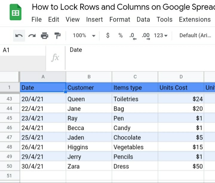
This is very useful when you have a lot of data inputted in a sheet. When you lock a row in your spreadsheet, it becomes visible as you scroll down to view other data in the spreadsheet. 

The top header or row becomes frozen on the sheet so that you won’t lose sight of which part of data you are looking for. Columns can also be locked on your spreadsheet. 

For instance, when you have a lot of columns on your spreadsheet, as you scroll to the right, you lose sight of the data that were on the previous columns, this is when you would want to lock your columns on your sheet so that the previous columns become frozen as you scroll left or right on your spreadsheet.

 Locking of rows and columns are done in two easy and quick methods, which are:

1.  Locking rows and columns with freeze panes in the toolbar or tab section.
2.  Locking rows and columns with freeze panes using the mouse.

 At the end of the guide, one would know how to:

1. Lock rows and columns on your Google Spreadsheet.
2. Protect an entire sheet in Google sheets.
3. Lock rows or cells and give Edit permission to selected people.
4. Show warning but allow editing of locked rows and columns.
5. Unlock a locked row or in Google sheet.

Method 1: Locking rows and columns with Freeze Panes using the toolbar or settings tab.

For Rows 

Step 1: Click on View.

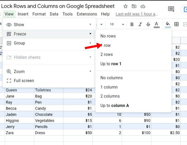
Step 2: Click on Freeze. It shows an array of options such as No row, 1 row, 2 rows and Up to current row.

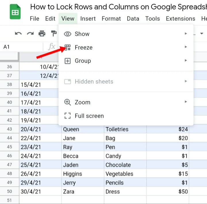
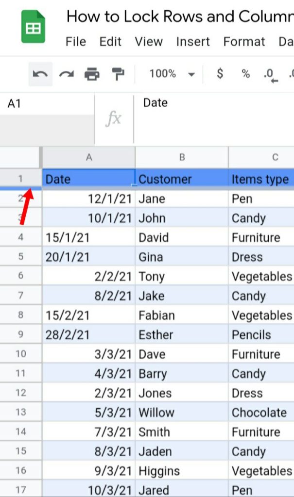
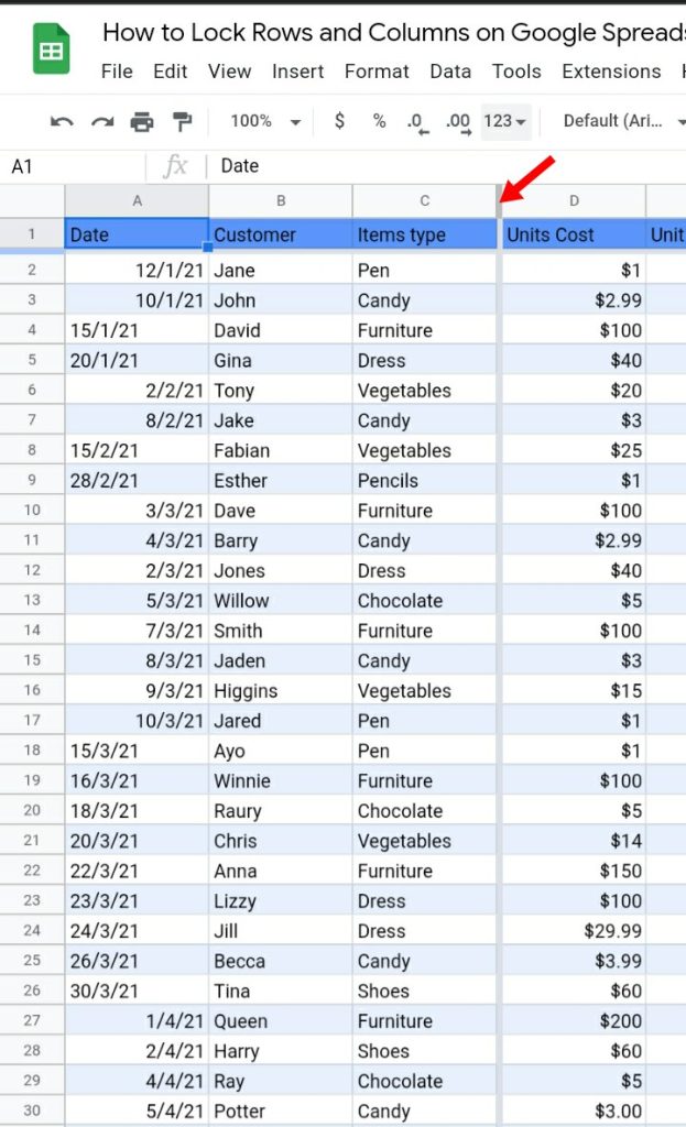
Step 3: Click on 1 row. It automatically freezes the first row, whereby the first row is highlighted and a gray thick line cuts through the row.

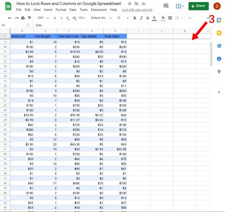
If you scroll down, you would notice that the first row or cell is still visible. This indicates that the row has been successfully frozen.

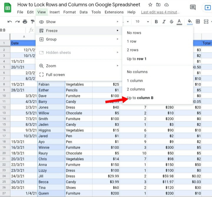
For Column:

Step 1: Select the column you want to freeze, it could be any of the columns in your sheet.

Step 2: Click on View.

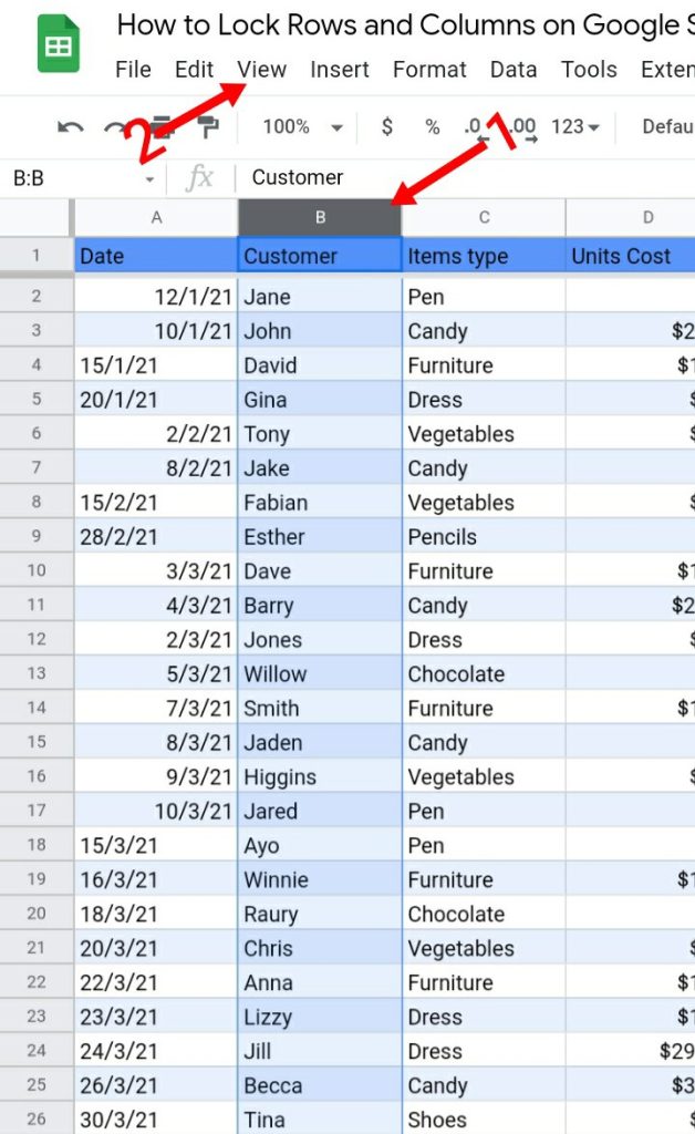
Step 3: Click on Freeze. It shows options such as No column, 1 column, 2 columns and Up to column B.

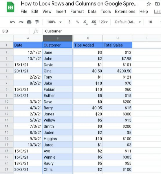
Step 4: Click In Up to column B. It automatically highlights the column, which indicates the column has been frozen.

If you scroll to the right on your sheet, Column B would still be displayed on the sheet.

Method 2: Locking rows and columns with freeze panes using the mouse.

This is the fastest and easiest method for locking rows and columns on your Google spreadsheet. It is easy to understand, operate and implement.

For Rows

Step 1: Move your mouse to the top left corner of your sheet. You would notice a gray box with two thick lines at the bottom and the right side. 

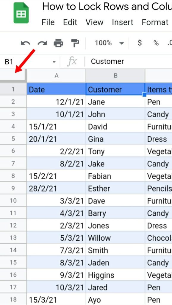
Step 2: Simply hover your mouse icon on top of the thick line below the gray box.

Step 3: Left click and drag the icon down below the row which you would want to freeze. I chose the first row so I can see the headers when scrolling down.

Step 4:  You would notice a thick gray line that cuts through the row. This indicates that the row has been frozen. You can scroll down to the last row on your spreadsheet but the first row or header would be visible.

For Columns:

Step 1: Move your mouse to the top left corner of your sheet. You would notice a gray box with two thick lines at the bottom and the right side.

Step 2: Simply put your mouse icon on top of the thick line at the right side of the box.

Step 3: Left click and drag the icon to the left, to any column you want frozen, drop it there and the column becomes frozen.

You can scroll to the left or right on your Google sheet but the column would still be displayed there, on the sheet.

How to Protect an Entire sheet in Google sheets.

If you don’t want some parts of the data inputted on your sheet to get erased, edited or deleted, you can protect any part of your sheet like a row or column which you don’t want to get edited. Here, we’ll show you how to protect an entire worksheet in Google sheets.

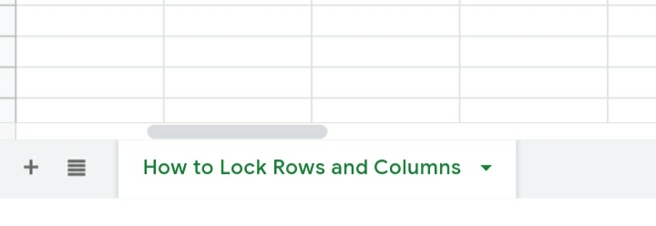
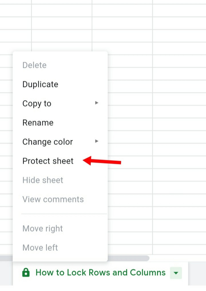
Step 1: Right-click on the name or title of the spreadsheet below the sheet. An array of options would appear on the screen.

Step 2: Click Protect Sheet.

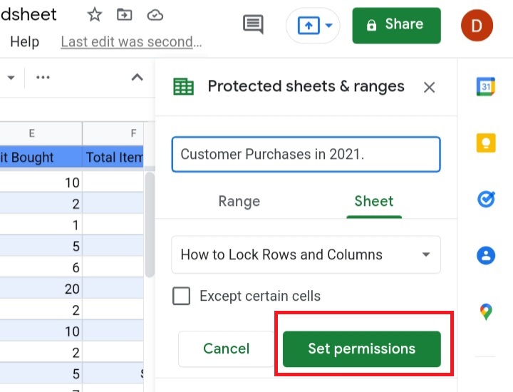
A pop-up by the right side of your sheet would appear, showing the description, the protected sheets and set permissions.

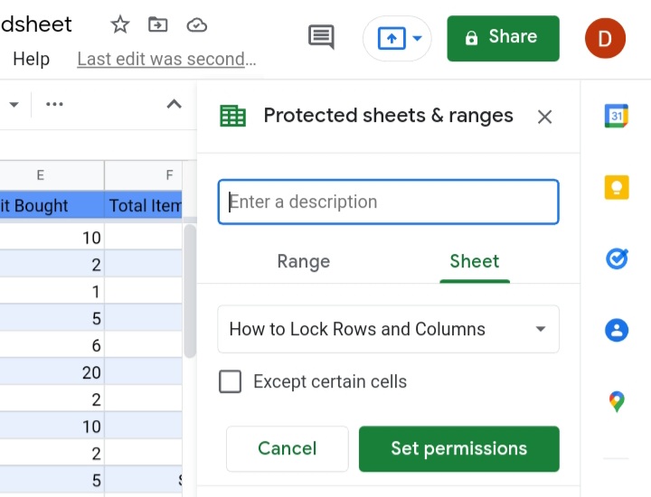
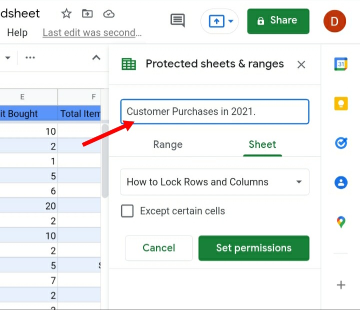
Step 3: Enter a description. This isn’t compulsory, you can decide to enter one or not. For example, Customer purchases in 2021.

How to Edit and Give permissions to selected people.

From the previous topic on how to protect our worksheets, we would continue how to edit and give permission to a selected number of people or colleagues.

Step 4: Click on Set permissions.

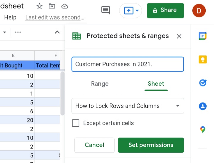
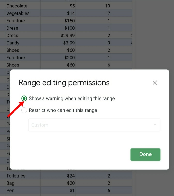
A pop-up would list the permissions you can grant on your sheet.

●      Show a warning when editing the range.

●      Restrict who can edit this range.

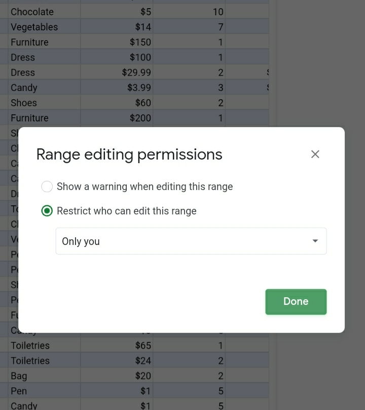
Step 5: Click on Restrict who can edit this range. This setting restricts editing from anyone else who is working on the same spreadsheet as yours.

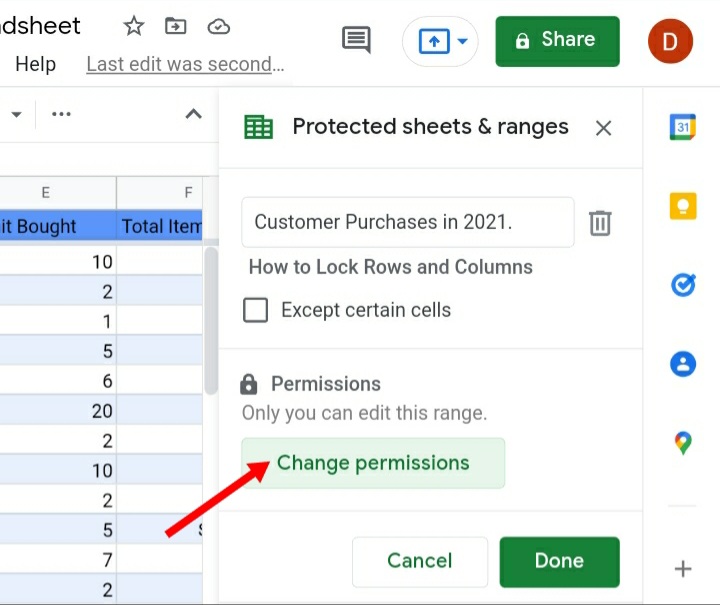
Step 6: Input the setting to Only you. This permits only you to edit the spreadsheet. Click Done.

If you want to change the permissions to grant access to a selected group of people, here are the steps.

Step 1: Click on Change permissions here to allow access to a set of people.

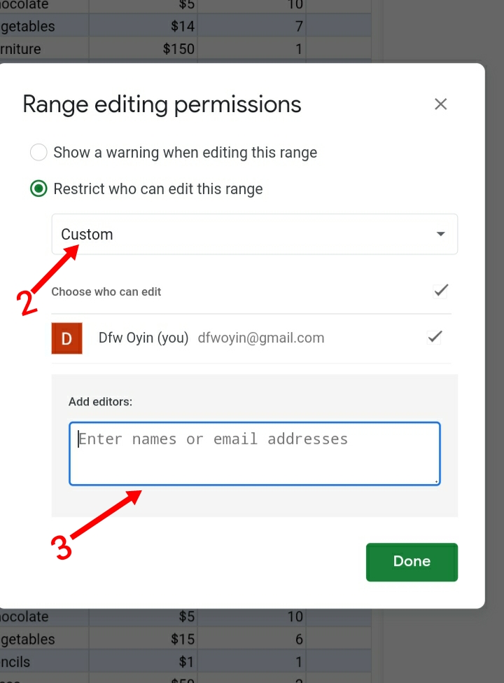
Step 2: Change from Only you to Custom.

Step 3: In the box below, you can add the names or email addresses of the selected people you want to approve to edit your google spreadsheet.

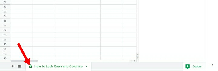
Step 4: You would notice a locked symbol in front of your spreadsheet’s title. This indicates that your sheet is protected.

How to Show Warning but Allow Editing on Spreadsheet.

This feature displays a warning whenever any row or column on the spreadsheet is about to be edited.

Step 1: Click on Set Permissions.

Step 2: Click on Show a warning when editing this range and click on done.

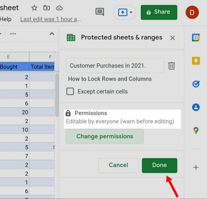
Step 3: The permissions show that the spreadsheet can be edited by anyone but it displays a warning before editing. Click on done.

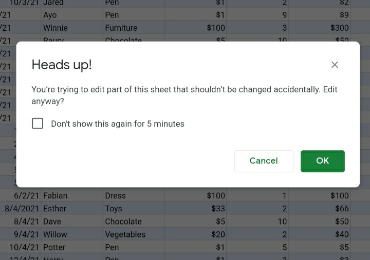
If any part of your spreadsheet (rows or columns) need to be edited or modified, it produces a heads-up warning below.

How To Unlock A Locked Row.

You can also unlock a range of locked cells or rows in google sheets.

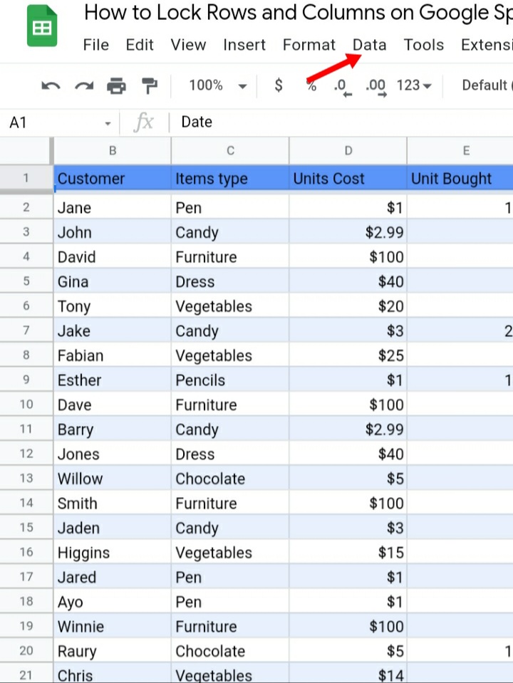
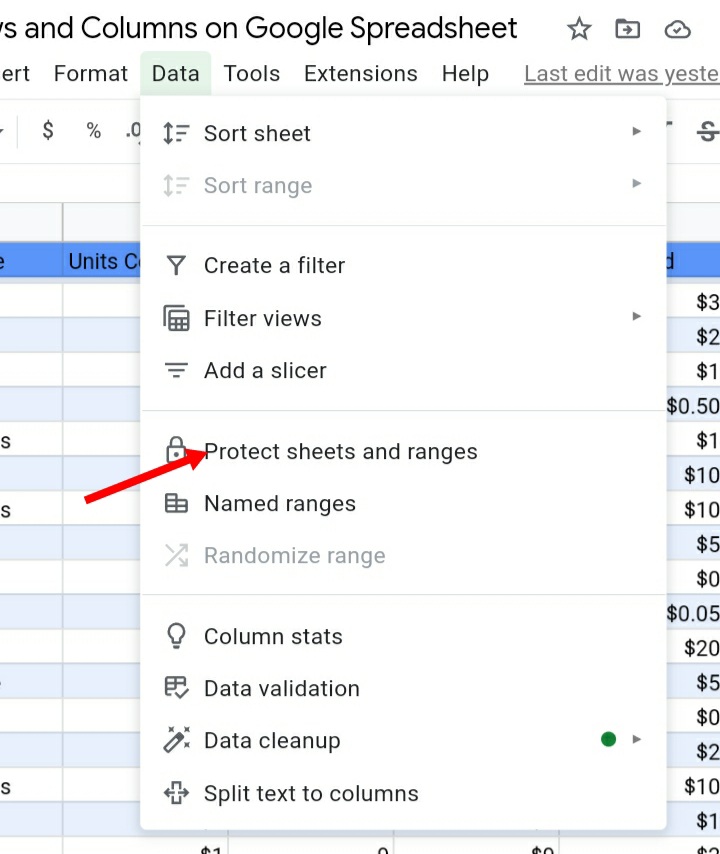
Step 1: Click on Data.

Step 2: Click on Protected Sheets and Ranges.

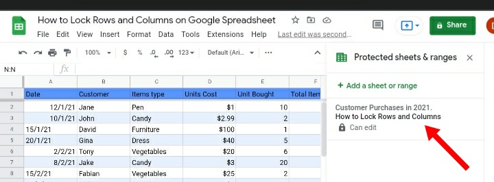
Step 3: On the right side of the screen, is the protected sheets and ranges tab. As you can see Customer Purchases in 2021 are locked and protected.

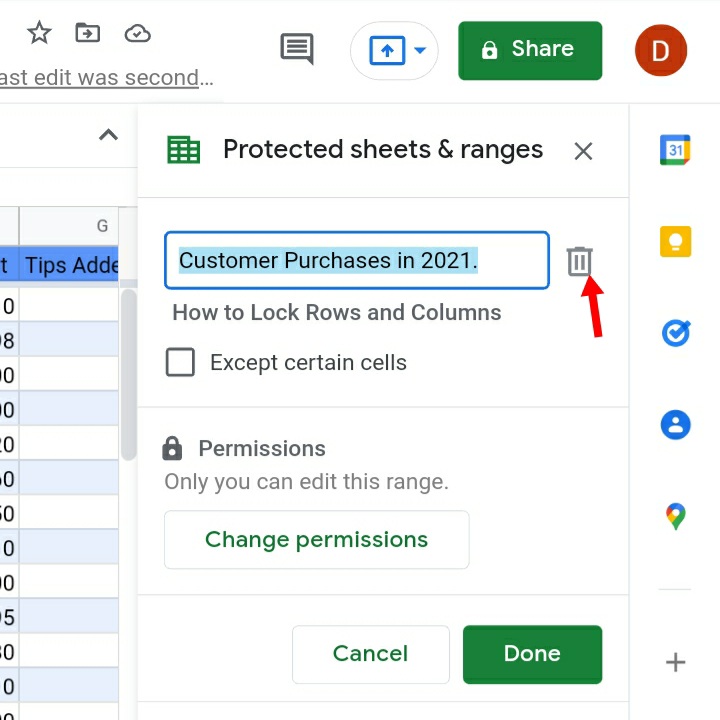
Step 4: Click on the recycle bin icon to delete the protection placed on the sheet.

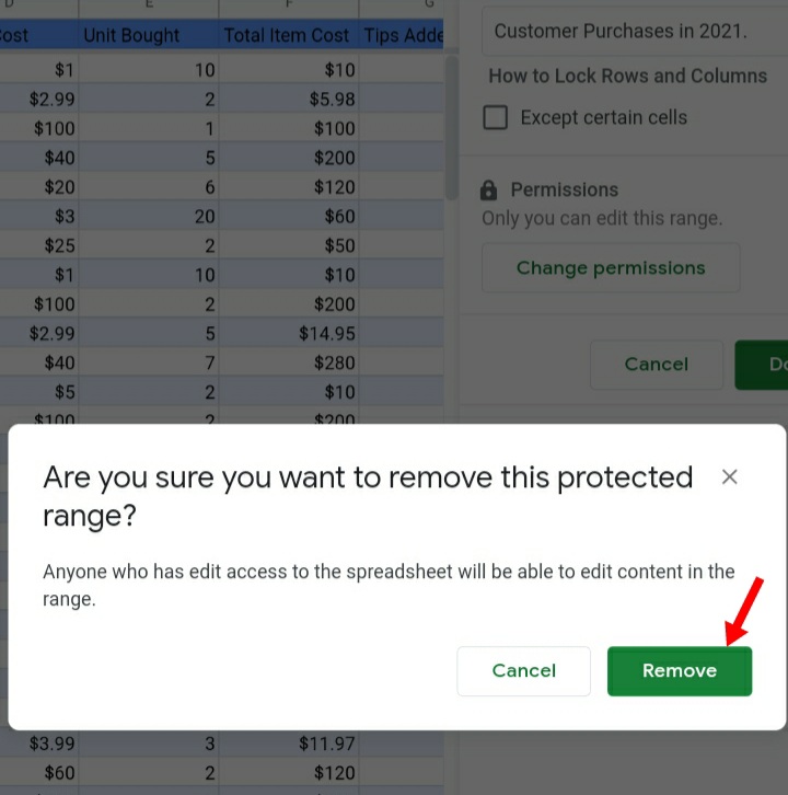
Step 5: A pop-up warning is displayed, asking if you are sure you want to remove the protection. Click Remove to confirm.

Step 6: You would notice the lock icon in front of the sheet title has been removed. This indicates that the spreadsheet is now unlocked and can be edited easily.

Why is it important to Lock rows or cells on my Google Sheet?

Locking rows and columns on google sheets are very easy but tricky to do. This is necessary when multiple people are inputting different types of data or changing formulas on the same Google sheet. 

You wouldn’t want them editing or deleting an important piece of information on your spreadsheet by mistake. Here’s where you lock your sheet’s data to avoid errors and omissions caused by a third party.

Conclusions:

Locking rows and columns of sheets help to prevent editing and deletion of important data. It also helps to keep tabs on headers or rows when working with large sets of data.