What if I gave you a way to make your job easier while still allowing you to better grasp the distribution of your data or to have some variance in it?
Wouldn’t it really save you time if your data is organized in such a way that you could figure out all of the answers to the most critical questions just by glancing at the information?
In this tutorial, I will show you a couple of ways to make negative numbers red in Google sheets. Creating patterns and trends in your data can be easily done with some simple techniques.
Grab a chair and let’s get started!
How to make negative numbers red in Google sheets
By the end of this tutorial, you will aware of marking negative numbers in red in Google sheets:
- Method 1: Make negative numbers red using Conditional Formatting
- Method 2: Make negative numbers red Using Custom Formatting
Both the methods will make your data highlight negative numbers red.
Method 1: Make negative numbers red using Conditional Formatting
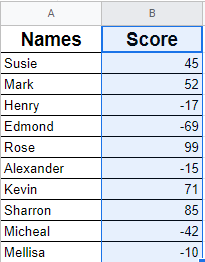
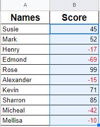
Suppose you have a database as shown below and you want to highlight the negative numbers mentioned in column B.
Below are the steps you can use to ‘mark negative numbers in red’:
1. Select column B i.e. Score column with the left click and drag down.

2. Right click on the column. You will find view more cell action select conditional formatting.
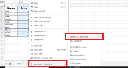
(OR)
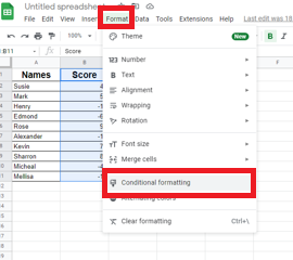
Click on the Format option on Menu Bar and select Conditional Formatting.
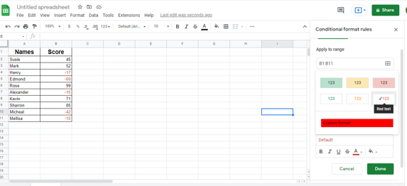
3. Once you select Conditional Formatting a dialogue box will appear called ‘Conditional Format Rules.’
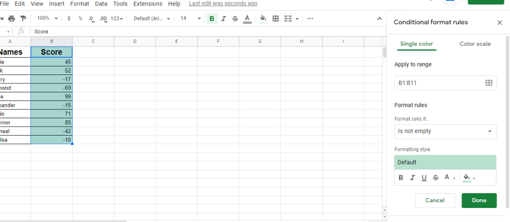
Apply to Range states which column(s) or row(s) you want to format. Format Rules are the rules applied to the selected range in the spreadsheet. It has myriad options along with custom formatting.
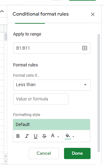
4. To highlight the negative number in column B i.e Score column, you will have to select the option under Format Rules >> format cells if >> Less than.
Check out the image below.
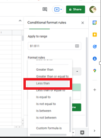
5. Once you select the Less than option, a small box will appear asking to add value or formula.
6. As we are required to format negative numbers in color red add the number zero in the value or formula box.
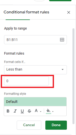
7. As soon you add the number zero you will find the negative numbers are highlighted with the default color.
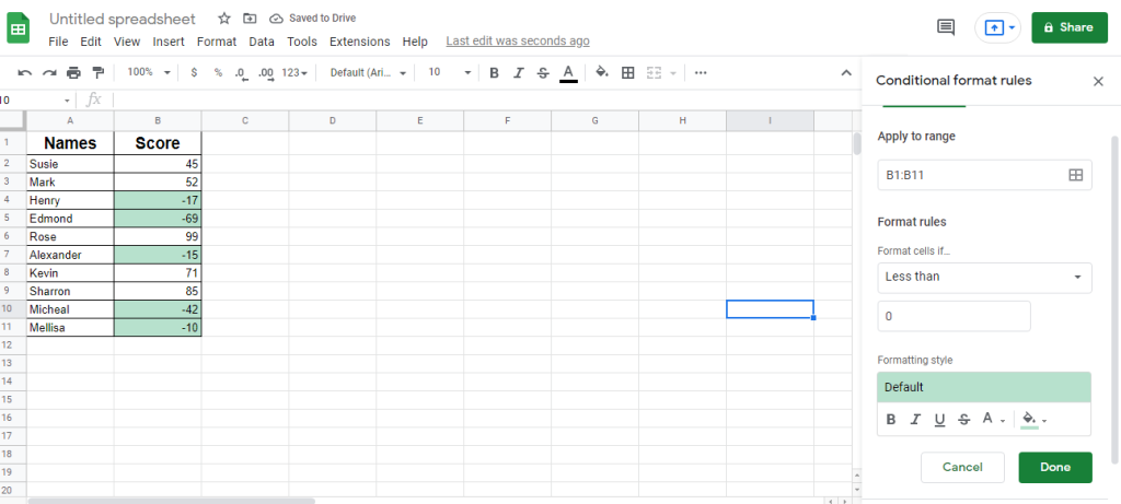
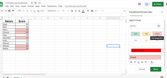
8. You can change the color by clicking on the default option and selecting a red color option or you can also select the red numbers option or the customized color red.
Check out the steps in the below picture to get a clear idea.
There you go! Now you can have any amount of list formatted as easy as a blink.
Let’s move on to the second method i.e.
Method 2: Make negative numbers red Using Custom Formatting
Below are the steps you can use to ‘mark negative numbers in red’:
1. Select column B i.e. Score column with the left click and drag down.
2. After selecting column B, click on the Format option on Menu Bar. Select Numbers >> Custom Number Format.
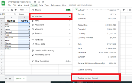
3. A dialogue box will appear called Custom number format.
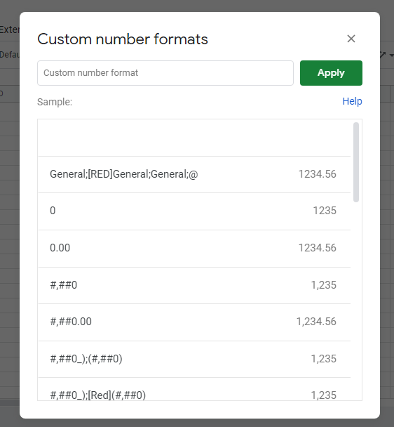
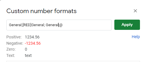
4. Add the format in the box – Customer number format and apply.
5. General is how you want the positive number to be shown after the 1st semicolon is how you want the negative number to be shown, the third part is how you want the zero values to be shown, and the last i.e. fourth part is how you want the text to be shown.
6. Once you click on apply, you will find all the negative numbers in Column B under the Score column that will appear in Red.
There you have your negative numbers marked in red in Google sheets in two different ways.
Extra Tip:
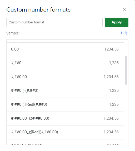
If you view carefully the below image, you will find # (pound/ hash sign) or 0 (zero). The # sign and 0 are known as placeholders of numbers. # (pound or the hash sign is the variable placeholder whereas 0 is a fixed placeholder. It is generally used to indicate decimals or thousand separators.
With these two simple approaches, you can now organize any amount of data in a matter of seconds with a few clicks.
Hope this tutorial was helpful for you to make you work effortlessly next time!


