Wildcards are very important tools used to search specific data in large worksheets. In this tutorial, we would show you how to use wildcards with three different methods to fully optimize the wildcard feature.
Definition of Wildcard Characters
Wildcards are characters that are used to illustrate one or more characters in a worksheet. These characters operate in collaboration with conditional, search, filter and lookup functions to generate more questions and search more dynamic. Three major wildcards used in Google Sheets are:
● Asterisk(*) – This wildcard symbolizes one character or several characters in your worksheet.
● Question Mark(?) – represents one character in the data.
● Tilde(~)- this wildcard operates in conjunction with other wildcard characters to notify the Google sheets operating system to identify the wildcards used in that context, as a normal symbol.
What are Wildcards used for in Google Sheets?
Wildcards are used to search and replace similar words in your worksheet. They are used to search texts containing a character or a group of unique characters or letters. Wildcards can be effectively used in three major ways.
- Using the Filter tool to filter data with wildcards.
- Using Wildcards with the SUMIF function.
- Using the Partial lookup or VLOOKUP function with wildcards.
Method 1: Using the Filter Tool.
This is done by creating certain conditions using the filter tool to produce values that match the given conditions.
For example, you own a fashion store that sells all sorts of designer wear, shirts, bags, and shoes and you would like to know the sales made on specific items, this is where you employ the filter tool to search and extract the data required.
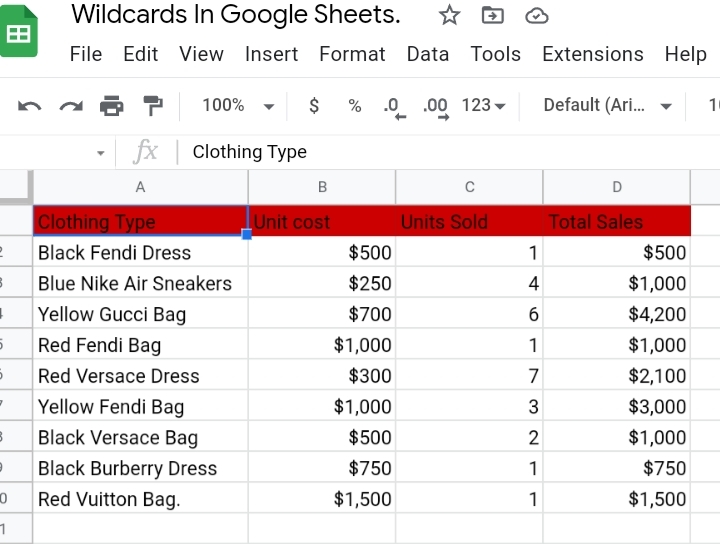
The filter tool is used effectively, following the steps stated below.
Step 1: Select and highlight the range of data on your worksheet.
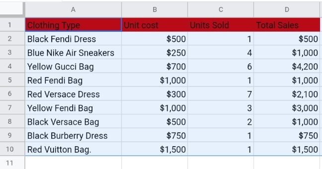
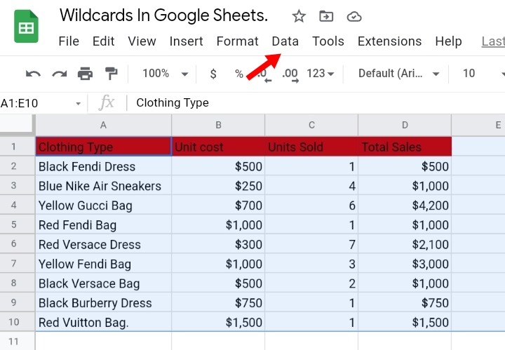
Step 2: Click on Data on the toolbar.
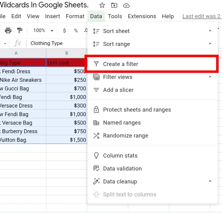
Step 3: Click on Create A Filter.
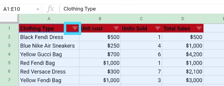
Step 4: A filter icon appears on the headers on your worksheet. Click on the icon.
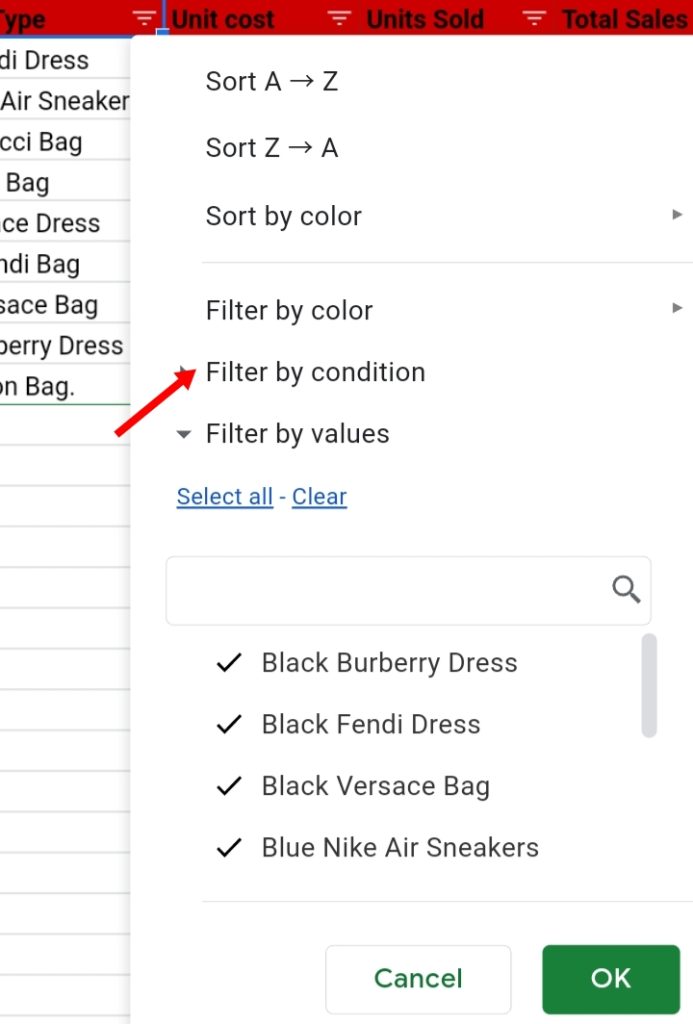
Step 5: A list of filters is produced. Select Filter by Condition by clicking on the drop-down arrow next to it.
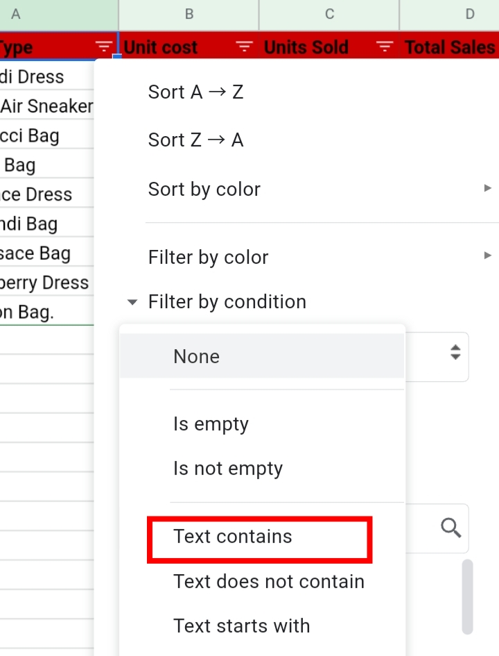
Step 6: Select Text Contains.
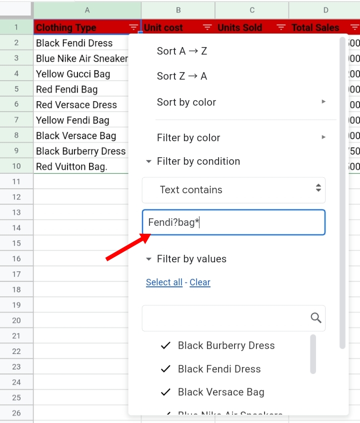
In the box, input your condition and a wildcard. For example, I want to filter the list of items and I only want to view the bags of the Fendi brand. Therefore, I would type the filter as Fendi?bag*
Step 7: Click OK.
Step 8: Now, it searches the dataset, filters and returns values that matched the specific set condition.

Method 2: Using Wildcards with the SUMIF function.
If you want to search for specific data and add its values, you could just search manually by scanning through with your eyes, but what happens when you have hundreds or thousands of data on your Google sheet?
Searching manually would be tedious and a waste of time. This is where the SUMIF function in combination with wildcards, saves the day!
By using the combination formula and listed steps below.
=SUMIF(cell range 1, ” *condition”, cell range 2)
Where;
- SUMIF adds the selected cell range IF it obeys your set condition.
- Cell Range 1 is the first column selected or column A.
- Cell Range 2 is the column containing the numerical values you want to add up.
- Condition is the factor considered for the selected ranges to be added.
- Asterisk(*) is the wildcard used in the formula.
Using the sample worksheet used in the first method, we would like to inquire about the total sales made on a particular commodity, by following the steps stated below.
Step 1: Input the formula =SUMIF(cell range 1, ” *condition”, cell range 2) into an empty cell, F2.
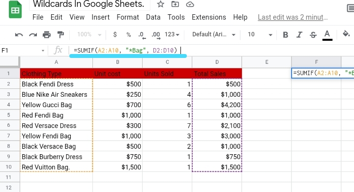
Step 2: Select cell range 1 (A2:A10) containing the item value you want to add.
Step 3: Set the condition in your formula. For example, I want to add the total sales made on the bags sold in the store. So, I set the condition as Bags.
Step 4: Select cell range 2 (D2:D10) containing the total sales made on each item sold in the store.
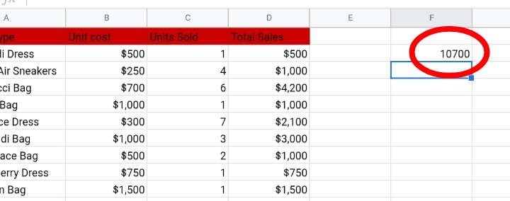
Step 5: Click Enter. The total sales made on all kinds and colors of bags are summed up in cell F2.
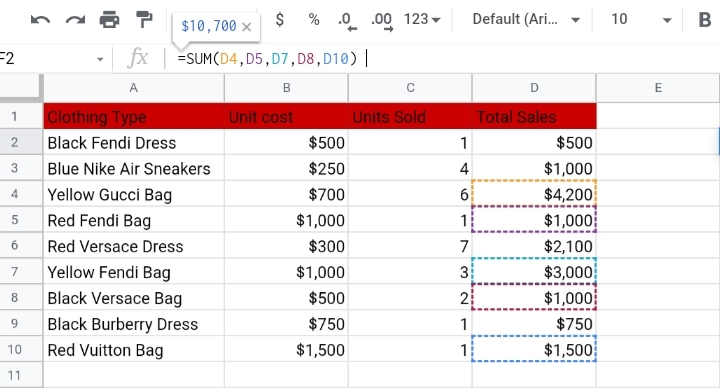
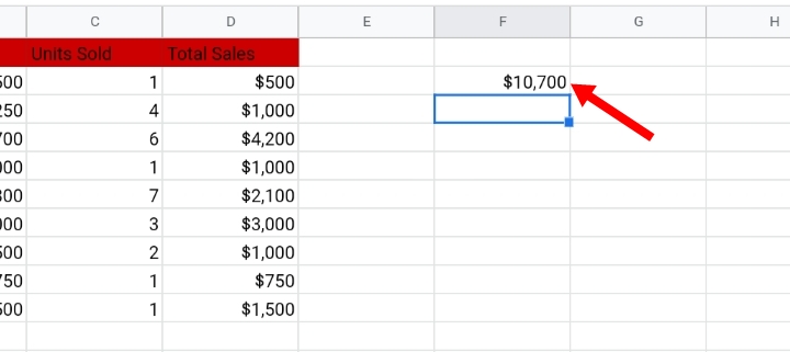
If you calculate the values manually using the basic SUM function, the total value of bags sold is the same as that of the SUMIF and wildcard result. This proves that this formula works effectively and accurately.
This also creates dynamic ways to search and sum products on specific conditions depending on what you want to extract from your dataset.
Method 3: Using the Partial lookup or VLOOKUP function with Wildcards.
First of all, what is the VLOOKUP function?
The VLOOKUP function is a search function used to scan the dataset for a value and return a matching value from whatever column you specify. It would only return values if it is an exact match but when placed with a wildcard, it produces partial matches.
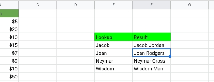
In this sample worksheet, a list of first names and surnames of people who donated for a fundraiser at an event.
Due to the long list of names, searching for details on the event is considered tedious and aggravating. This is where the partial lookup function eases stress and aids accountability.
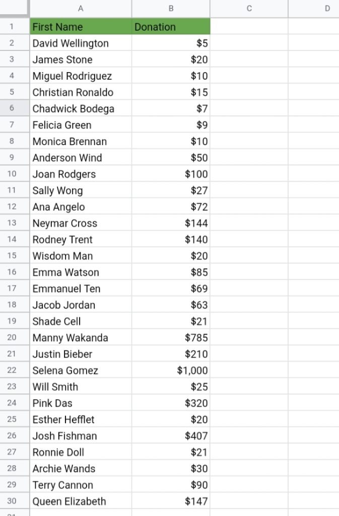
Using the formula and steps listed below, a partial lookup is done on the data set.
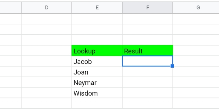
Step 1: In cell E5, create a table of the data you want to look up and the results.
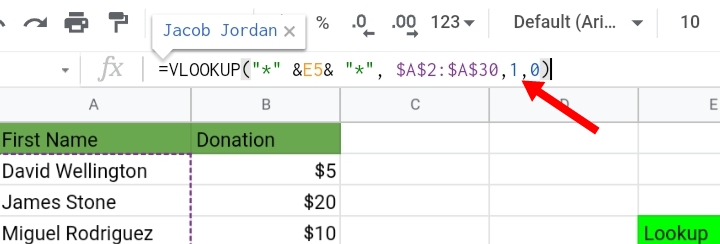
Step 2: Input the formula into cell F5 =VLOOKUP(” * ” &E5& ” * “, $A$2:$A$10, 1, 0)
The presence of the wildcard (*) in the formula made sure the VLOOKUP function searches for any text in the dataset that matches the word in E5.
Step 3: Click Enter and the matching data is entered in F2.
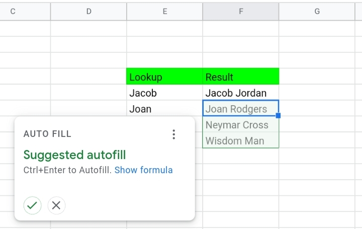
Highlight the remaining data and double click to auto-fill the results in the column.
Use case of the Tilde Wildcard in Google Sheets.
Although this wildcard is not used often, it is important to learn how, where and when it should be used.
For example, the worksheet below contains a list of words and characters in which the word s*m is amongst them.
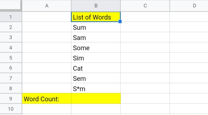
The formula below uses the asterisk wildcard to get the texts that start with the letter S and ends with M.
=COUNTIF(B2:B8, ” S*M “)
Step 1: Input the above formula in the Word Count row whose cell reference is B9.
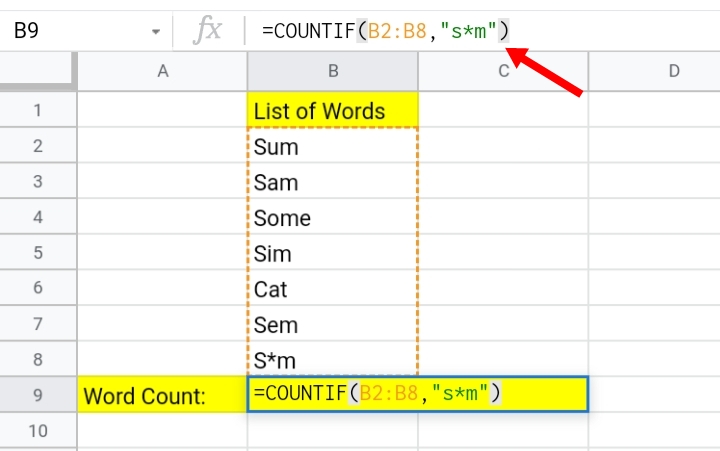
Step 2: Click Enter. Notice that the result generated below is not what we want here.
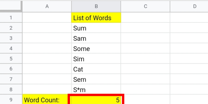
This is because the COUNTIF function identifies the asterisk as a wildcard and not an ordinary symbol. Therefore, every cell containing a word starting with the letter S and ending with an M in column B counts as a match.
To make sure the COUNTIF function counts only cells containing the word “S*M” the tilde wildcard is employed in the formula. Therefore, the formula in step one is replaced with a new one which is typed in cell B9 like this:
=COUNTIF(B2:B8, “S~*M”)
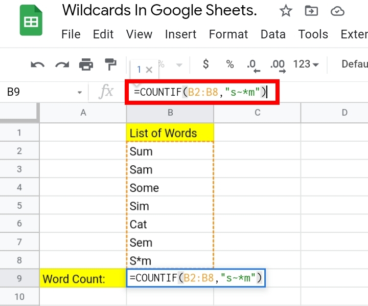
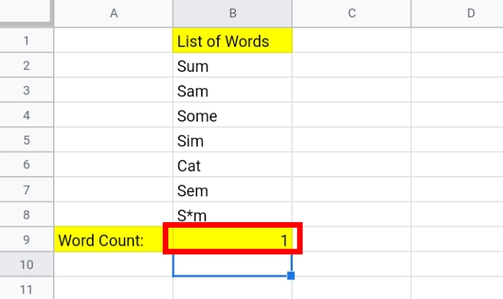
Click Enter. An accurate result is produced. Now the result would be given as 1 since only one cell contains the exact character, s*m.
Conclusions
With the three easy steps provided and explained above, we hope you’ve fully understood how to employ wildcards when you need them and how to use them for dynamic searches on your Google Sheet. I hope you enjoyed this tutorial, thanks for reading.


