A pivot table is a powerful tool used in Google Spreadsheets. It is mostly used for analyzing, summarizing, calculating statistical operations such as sums, total average etc. reorganizing and regrouping a set of given data.
A pivot table is a table composed of several rows and columns that can be moved around. It is a flexible power tool that also highlights similarities, significance, patterns and reveals information in a group of given data.
In as much as it is a powerful and effective tool, it poses a difficult task of construction and operation.
New business owners and beginners in the data entry and input field face difficulties when constructing a pivot table.
Some intermediate levels of workers also require a detailed process on how to input and construct an efficient pivot table.
This guide is aimed not only at newbies but also at average workers to level up and build their pivot table skills and their digital data skills as a whole.
HOW TO CREATE A PIVOT TABLE WITH GOOGLE SHEETS.
At the end of this guide, one would be able to
- Create a pivot table with ease and dexterity.
- Perform simple statistical calculations such as a sum of data, average cost, total goods sold annually etc. Depending on the type of data given.
It is advised to pay attention to this guide, to create a pivot table and display your data values successfully.
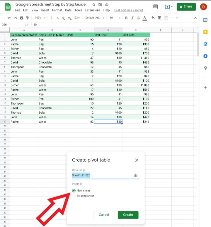
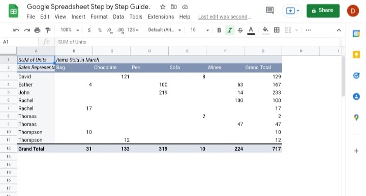
Here is the given set of data we would be working with to create a pivot table.
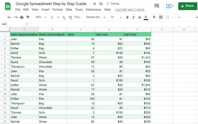
As you can see, the presented data above shows the sales made throughout March by a group of sales representatives in a store.
The sales records presented are disorganized, voluminous, filled with different trends and patterns which makes them rather difficult to understand. Here’s when we create a pivot table to summaries, simply and enhance the flexibility of the presented data.
Creating a Pivot Table.
With the well-detailed steps below, creating a pivot table would be made easy.
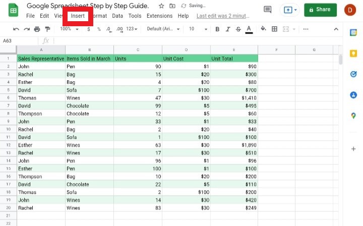
1. Click on the Insert button here.
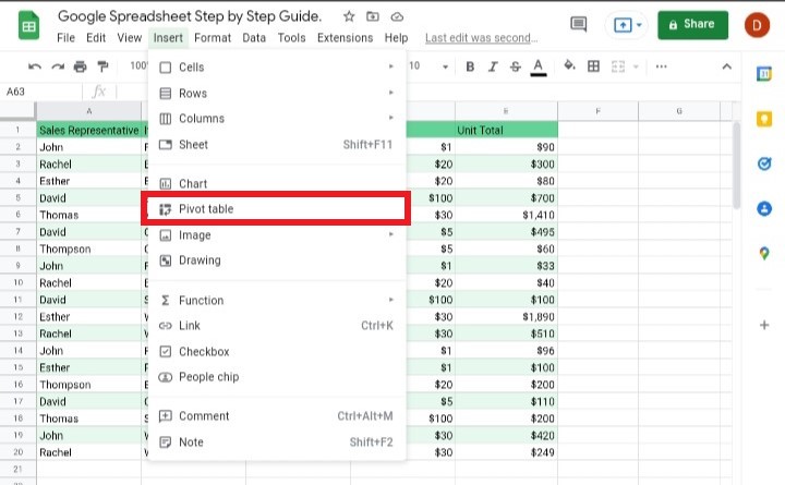
2. A list of options would be displayed. Click on Pivot Table here.
3. When you click on the pivot table, you would be asked to select a date range. Notice the square icon by the side, click on it. It is advised to use the suggested data range, as it automatically selects all the headers and data in your spreadsheet.
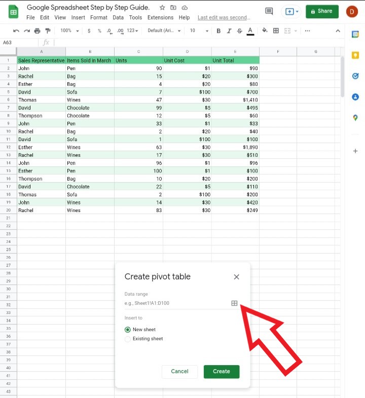
4. Click on New Sheet. This provides a fresh pate where the Pivot table would be created.
We can also click on the existing sheet, but the pivot data would be on the same sheet as the presented data which makes it a bit jam-packed and might cause confusion for users that are beginners. Therefore, it is advised to choose a new sheet to create your pivot table.
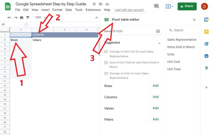
5. A new sheet is created, consisting of rows and columns. The rows and columns are used to highlight similarities between two variables on the given set of data.
The Pivot Table Editor is placed at the right-hand side of the table. This would be used to add rows, columns, values and filters to the pivot table. It automatically has an idea of the statistical analysis that may be used in the pivot table.
Some examples of rows, columns and Pivot Table Editor.
- Rows
- Columns
- Pivot Table Editor.
Check out How To Make A Table In Google Sheets (Full Details + Image).
How to Sort Rows on a Pivot Table In Google sheets
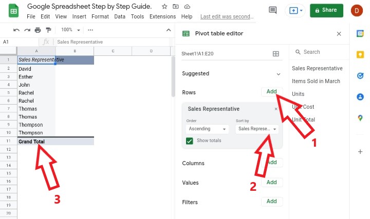
We would decide what type of information we want to input here.
1. Click on the Add.
2. Sort the rows by selecting a header. For example, I selected the header for the row to be for a Sales Representative. You can choose anyone from the list of headers given in your data.
3. On the left-hand perspective, you would notice that all the names of the sales representatives were listed out in ascending order. You can change the order as well by clicking the option.
You have successfully sorted out the rows of the Pivot table.
How to Sort Columns on a Pivot Table In Google sheets
We would choose what sort of information we want to display as the columns.
1. Click on Add.
2. Sort the columns by selecting a header. Note that; more than one header can be selected depending on the data and information you want to display.
For example, I selected the header for the column to be Items Sold in March.
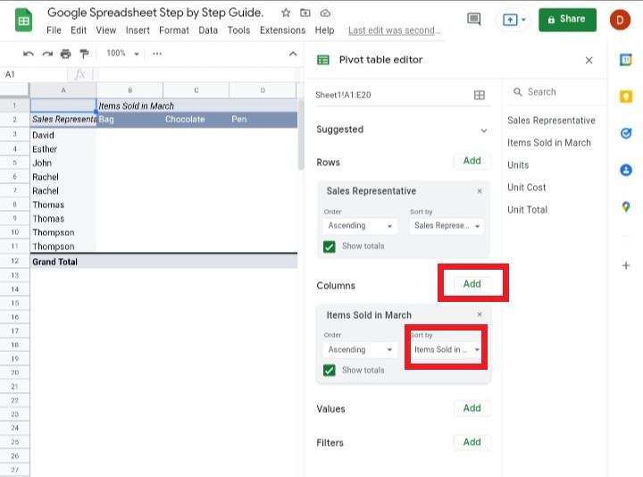
3. At the left-hand side of the screen, a pivot table has been created, displaying the types of Items sold in March, the number of items sold out, the names of the sales rep who sold the items and the total number of items sold in March. The pivot table calculates all the data in between.
If you’ve followed the steps correctly, you would have successfully inserted the column in your pivot table.
How to Sort Values on a Pivot Table In Google sheets
This is where the operator would like to determine the values or the numbers. All statistical operations take place here.
1. Click On Add
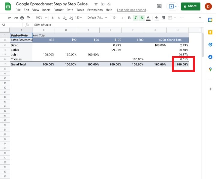
2. I decided to summaries the column using SUM, presented in a percent format, where the data would be displayed in percentage.
3. More than one value can be inputted, so I decided to add another SUM value in the default setting, where the data would be displayed in the numeral format.
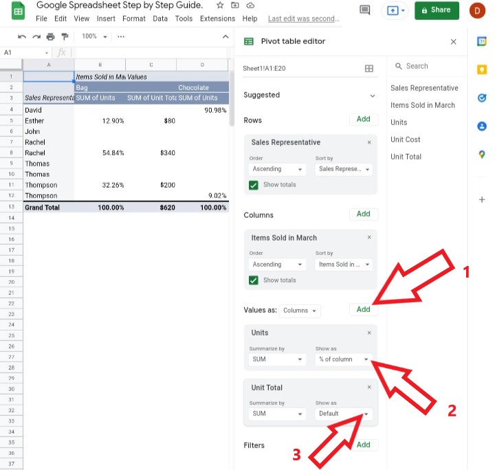
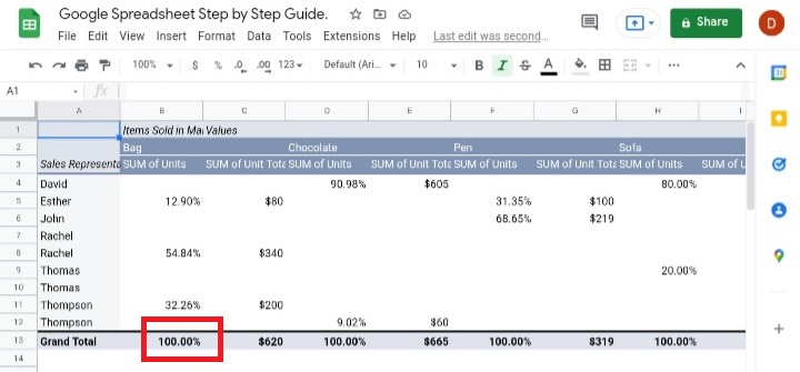
4. The pivot table presents the data, both in the percentage of the sum and the total of units sold.
How to Filters a pivot table in google sheets
Filters are used to sort out a particular set of information you only want to display.
For example, if the owner of the store wants to view items sold at prices at $100 and which of the sales representatives sold the items, he uses the Filter option on the pivot table.
1. Click Add
2. Select how you want to use the filters, either by a condition or by values.
3. The business owner would want to check the items sold at $100 and who sold them. Therefore, he only selects the $100 option.
4. Click on Okay.
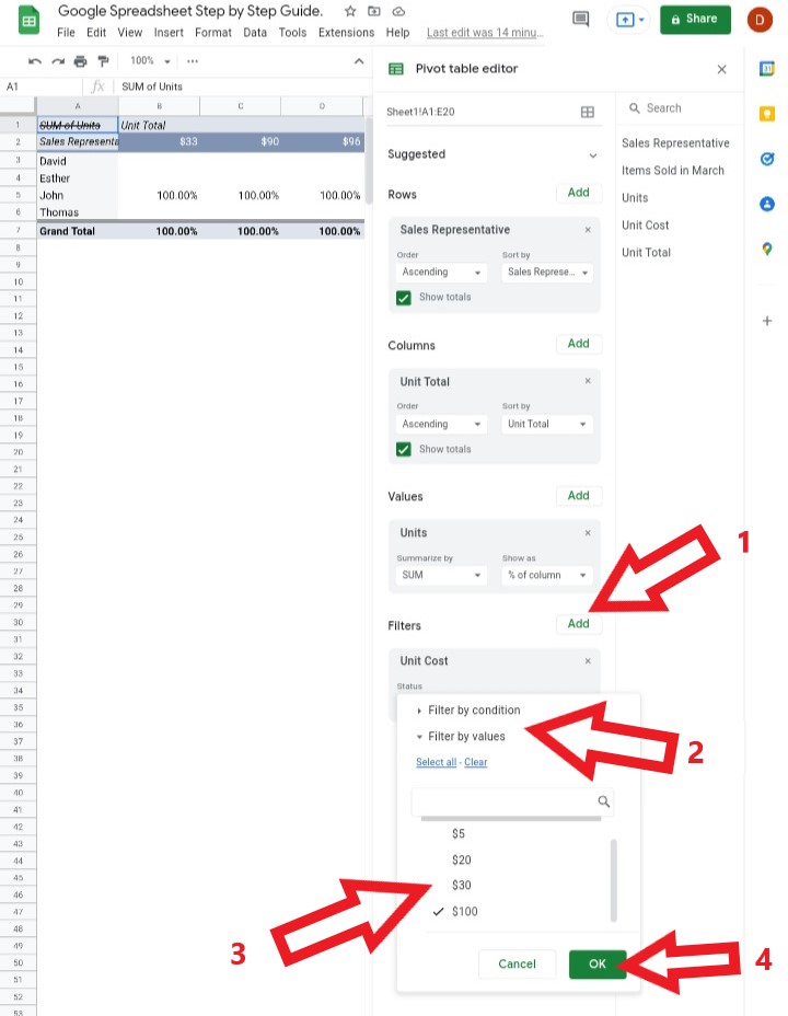
5. The pivot table filters the data and presents the items sold at $100 and the sales rep who sold the goods in a total percentage, as seen below.
Final Thoughts:
With this step-by-step guide on how to successfully create a pivot table, sort it with different values, row, columns etc. new business owners and data entry personnel would find it easy and task-free.
More information on your data would be revealed in a very flexible way.
Statistical operations and calculus have been made effortless and less tedious.


