Google’s Sheets storage capacity is very dynamic and can store and process multiple data types at a go. However, the more data type stored, the more challenging, finding and extracting data manually would be.
Searching each value manually with your mere eyesight would be stressful and cause fatigue.
Thankfully, Google Sheets has developed a search feature which enables us to find and replace all sorts of values in our worksheets.
In this tutorial, we are going to learn how To Search In Google Sheets. You can do your search within few minutes by using method describe in this article.
Search Using the Find Option To Highlight All Matching Cells In Google Sheets.
This method is preferably used when you want to find cells with a specific value to see the included data or to spot duplicates in your worksheet.
When the matching cells are spotted you can choose to highlight them to aid visibility and quick search.
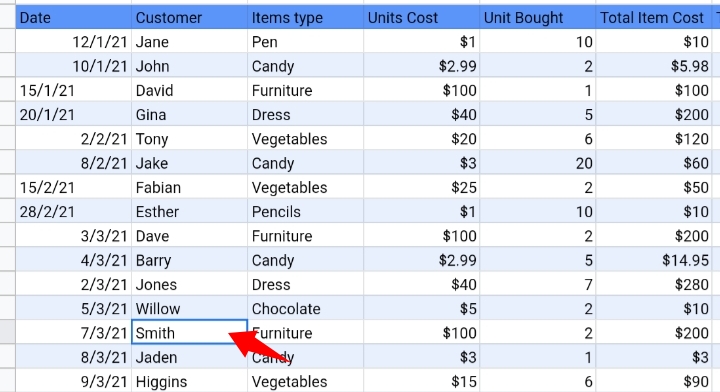
Using the sample worksheet below, we have a list of customers, the items bought, the unit price and the total cost bought. So we want to highlight the cells with the name “John”.
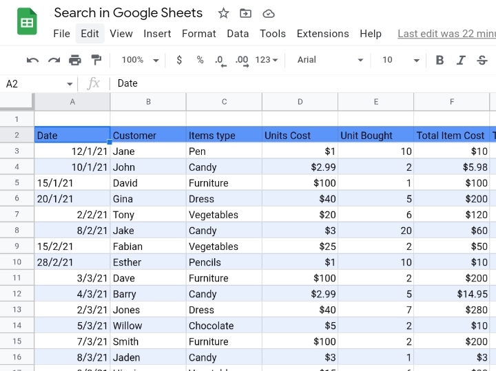
To do this, you’d have to follow the stated steps below.
Step 1: View the worksheet with the dataset you’d want to work with.
Step 2: You can use the shortcuts to open the find tab. These shortcuts are Ctrl key + F (Windows OS) and CMD key + F (Mac OS).
Step 4: The Find box is opened at the top right corner of the worksheet. In the box, we’ll enter the name we are looking for, that is John.
Step 5: Hit the Enter key and the cells with the name “John” are highlighted.
To scroll through the matching cells, simply click on the upward and downward arrows in the find tab. Also, you can manually scroll the highlighted cells and see them.
They tend to stand out from the other cells due to their added color. This method is quite quick and reliable. You can easily access and view the matching cells one at a time.
Search Using Find And Replace.
This is another method used to search and locate data on your worksheet. In a case where you require more access and management over the search key and results found, this method is very suitable for this.
Using the previous sample worksheet, let’s assume there has been an error with a customer’s name. A wrong name, Jane has been inputted in place of Janet.
So we would use this feature to find all occurrences of Jane and replace them with Janet. To do this, we need to follow the steps stated below.
Step 1: Navigate your way to the toolbar and click on the Edit option on the toolbar.

Step 2: From the drop-down list produced, select Find and Replace. Alternatively, you can directly use the keyboard shortcut, Ctrl key + H(Windows OS) or Command key + H(Mac OS) to open the Find and Replace tab.
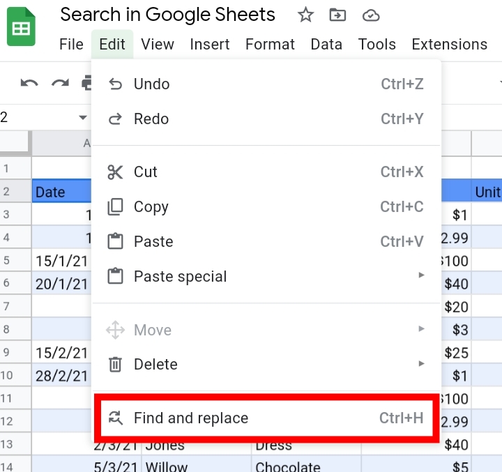
Step 3: In the textbox directly beside Find, input the text string we want to search for. In this case, it is Jane.
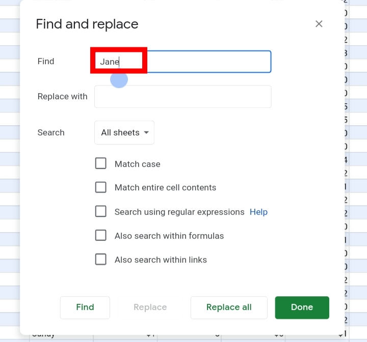
Step 4: In the Replace With section, type in Janet, since that’s what we want to replace the matching texts with.
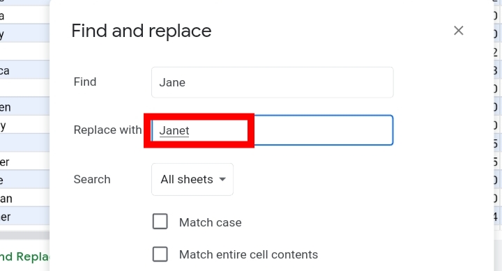
Step 5: Under Search, click on the drop-down arrow here. Click on Specific Range. Then, you enter the entire range of the worksheet in the textbox, close to it.
Step 6: There are five tick boxes with options. Select the first three options which are Match Case, Match Entire Cell Contents and Search using regular expression.
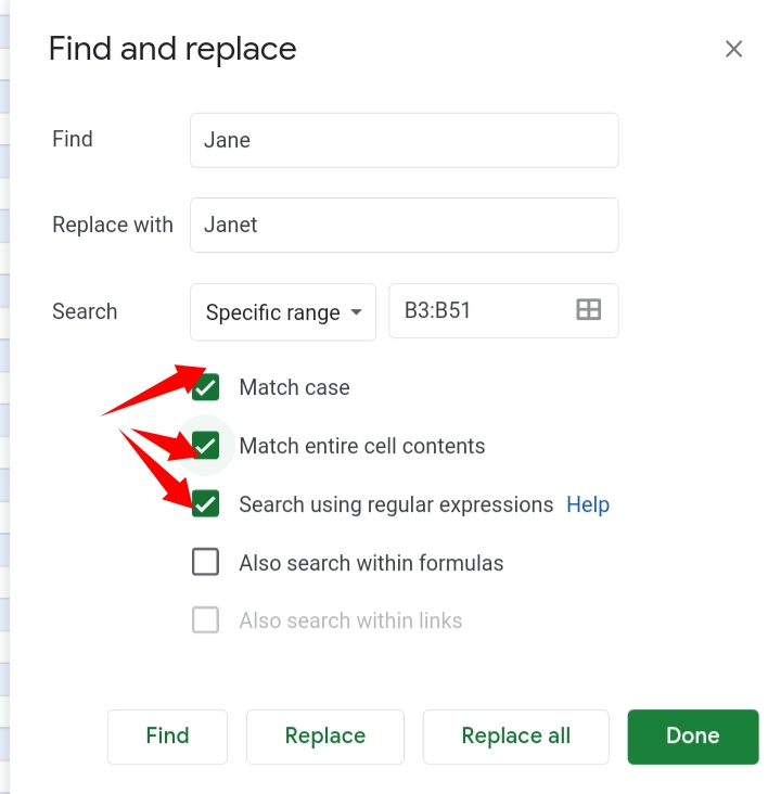
Step 7: Click on replace all.
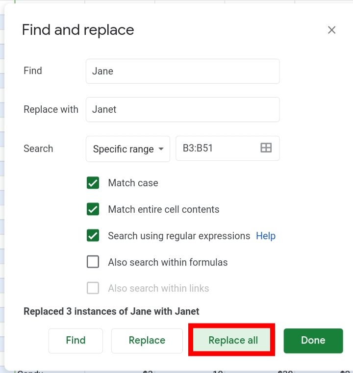
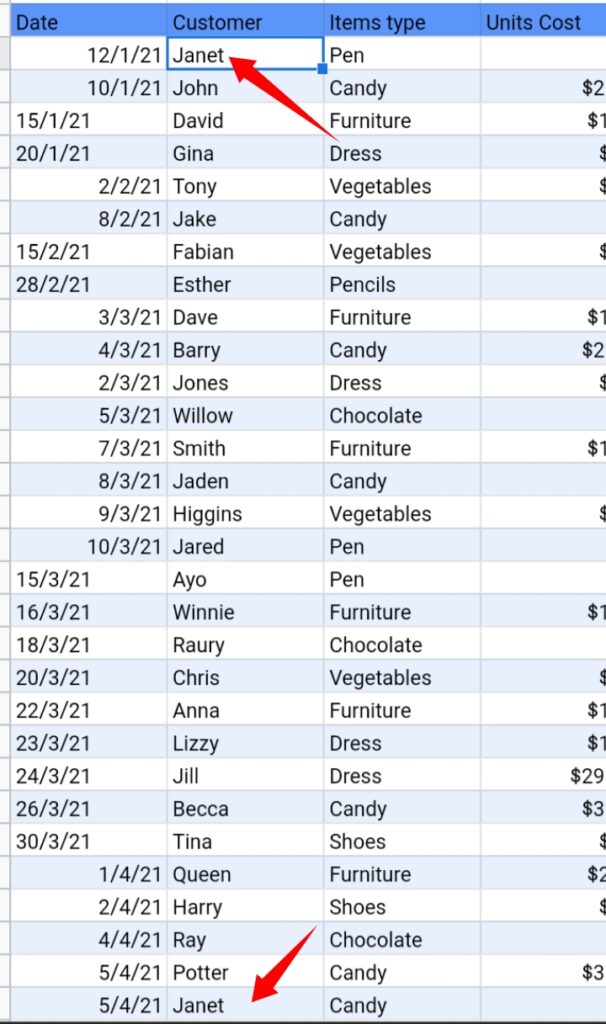
The feature finds and replaces each instance of Jane with Janet.
Search Using Conditional Formatting.
This is a more advanced method. It doesn’t involve the replacement of data. In a case where we can highlight a single or entire row that has one matching cell with the search key.
This is done by using conditional formatting.
First, we would learn how to search and highlight a single matching cell. It is done in the steps stated below.
Step 1: Select an empty cell. This is where the search key would be entered. In this case, we selected cell B1.
Step 2: Select the entire cell range of the data containing the search key and the matching data.

Step 3: On the toolbar, select Format.
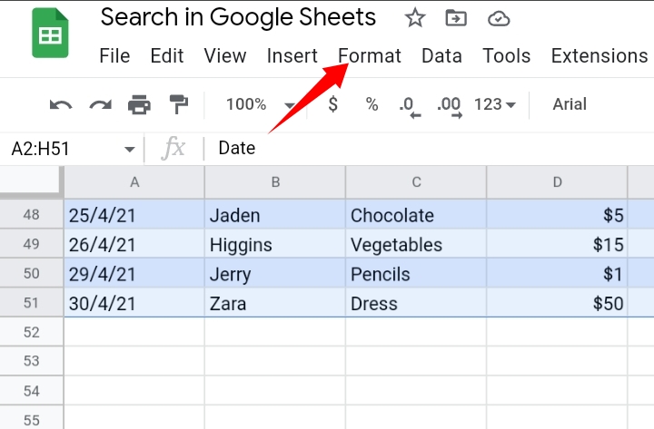
Step 4: From the drop-down menu, select Conditional Formatting.

Step 5: The conditional formatting tab is opened. Under the Format Cells If section, click on the drop-down arrow and select Custom Formula Is.
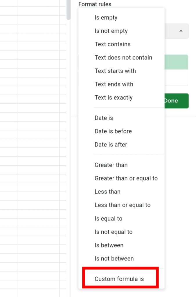
Step 6: Input the formula =B2=$B$1 in the Value Format textbox.
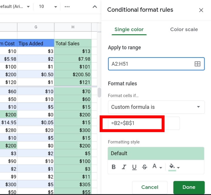
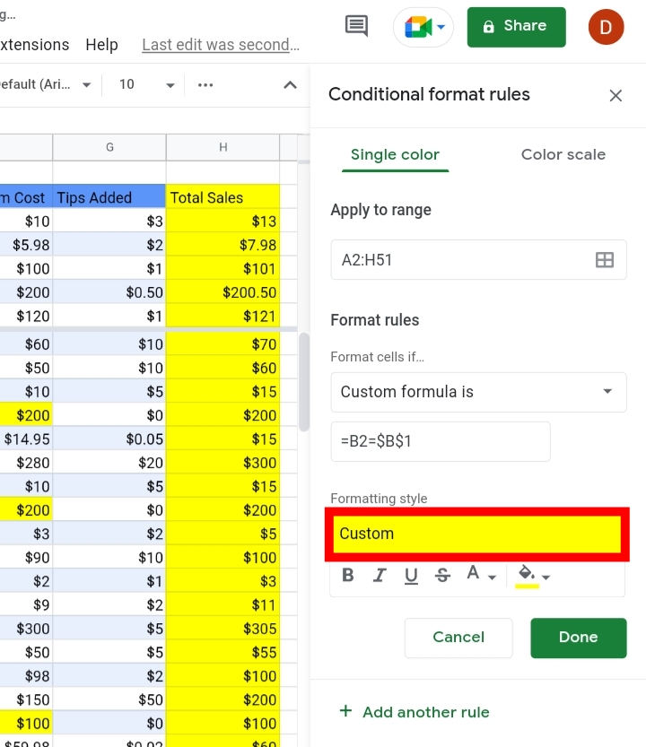
Step 7: You can customize the format, style and color. Here we selected yellow as the highlight color.
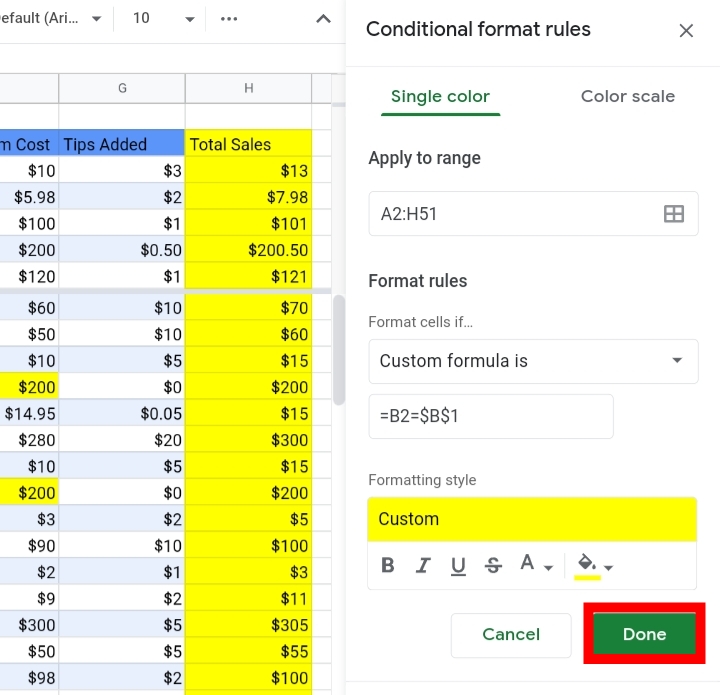
Step 8: Select Done.
Step 9: Now, enter the search key in cell A1. Here, we entered Jane.
Now, the matching cells in the dataset are highlighted in the worksheet.
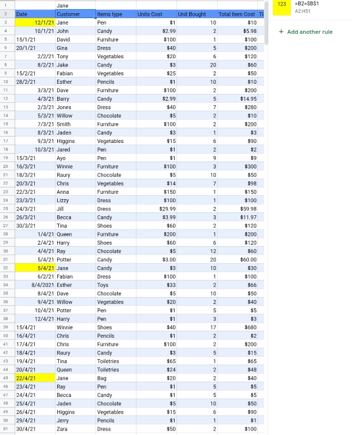
We know how to search and find the single data in a worksheet. What if we also want to see the entire row of the matching data?
To do this, we need to follow the steps below.
Step 1: Select an empty cell. This is where the search key would be entered. In this case, we selected cell B1.
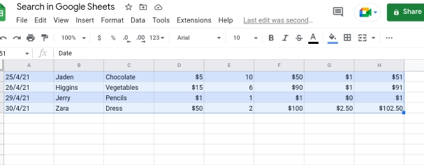
Step 2: Select the entire cell range of the data containing the search key and the matching data.
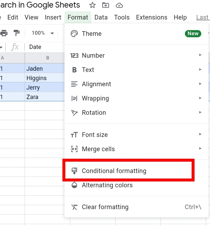
Step 3: On the toolbar, select Format.

Step 4: From the drop-down menu, select Conditional Formatting.
Step 5: The conditional formatting tab is opened. Under the Format Cells If section, click on the drop-down arrow and select Custom Formula Is.

Step 6: Input the formula =$B2=$B$1 in the Value Format textbox.
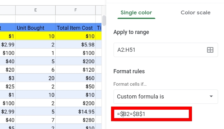
Step 7: You can customize the format, style and color. Here we selected yellow as the highlight color.
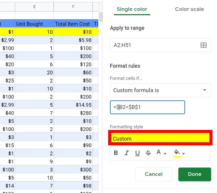
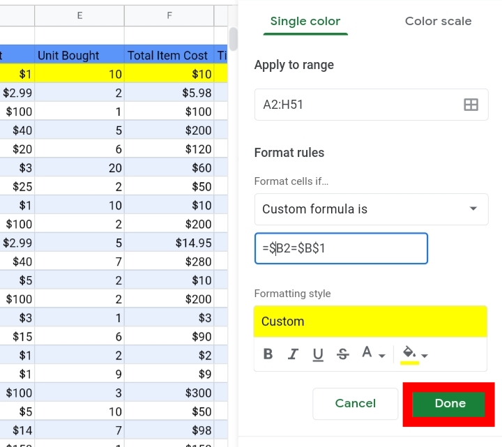
Step 8: Select Done.
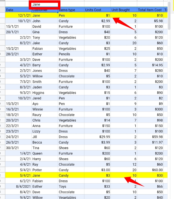
This way, we have a clear view of the other rows relating to the matching cell.
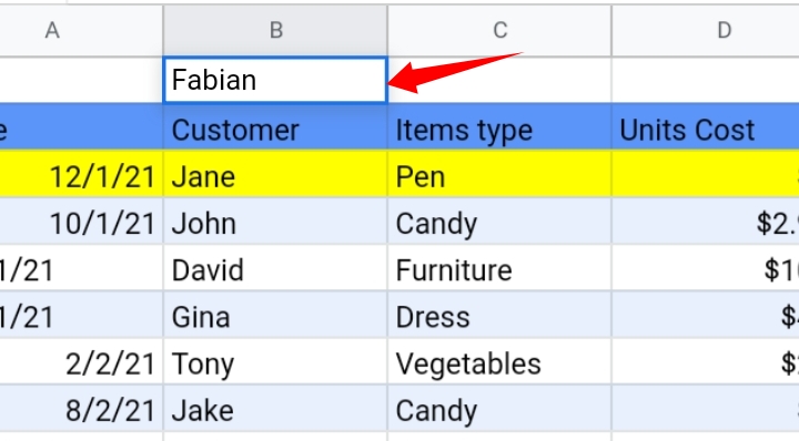
If the text is changed in cell B1, the highlights would change too.
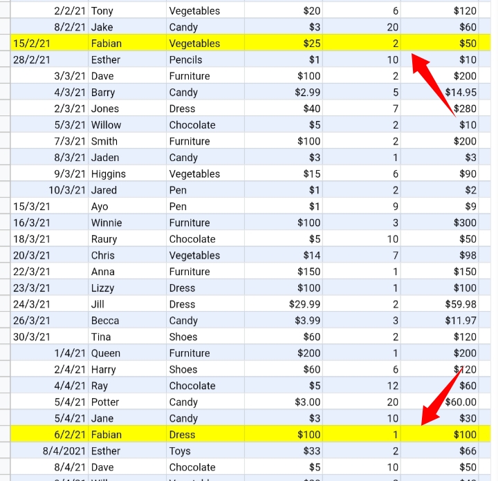
In a case where you have a large data set, you can create a dropdown menu using Data Validation so that all names and options are more organized in a list.
How To Search Values in The Google Sheets iOS and Android App.
The Google Sheets Mobile is limited in its features and functions unlike the Desktop site but it does have the Find and Replace feature.
Now, we will show you how you can use this feature on the mobile Google sheets app.
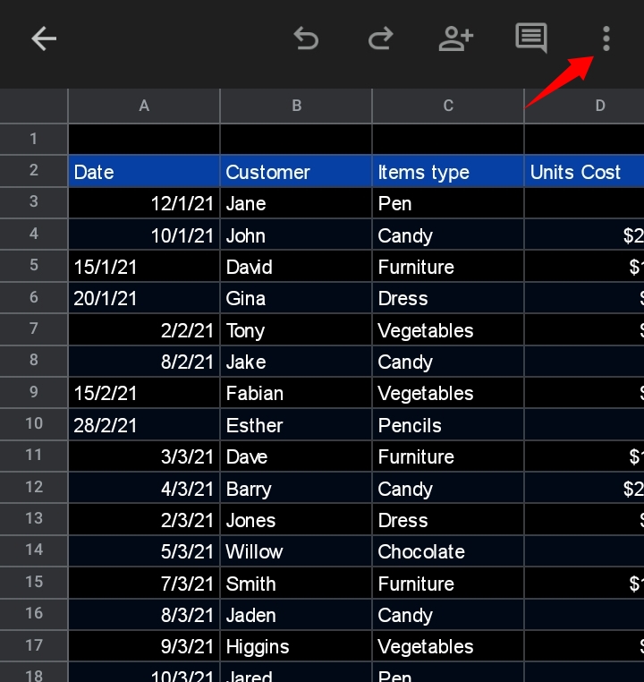
Step 1: Open the worksheet you want to work on. On the top right corner of the page, click on the three dots vertically arranged there.
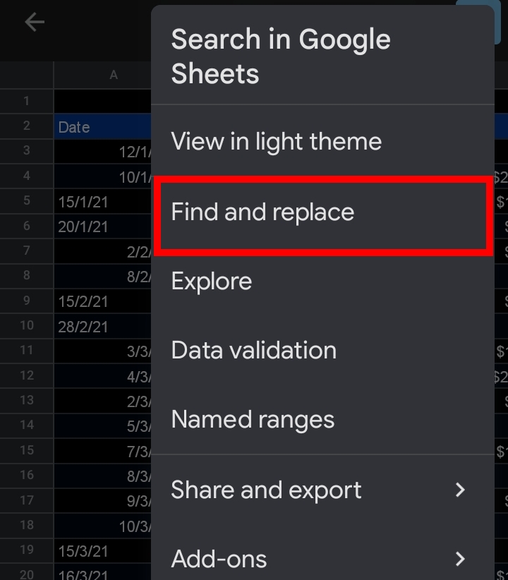
Step 2: A menu comes up. Select Find and Replace there.
Step 3: Enter the search key in the textbox and hit the enter key on your keyboard. Multiple matches are generated for you.
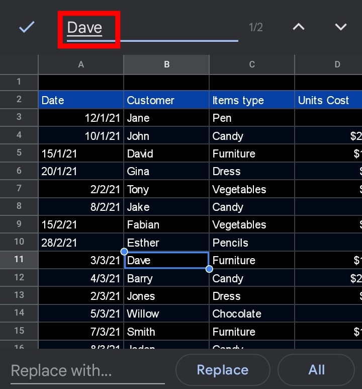
Step 4: Click on the arrows at the top right corner of the screen to view each generated match of the search key.
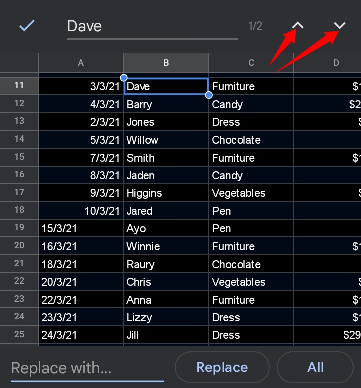
Step 5: To replace the matching cells, enter the replacement text and select Replace.
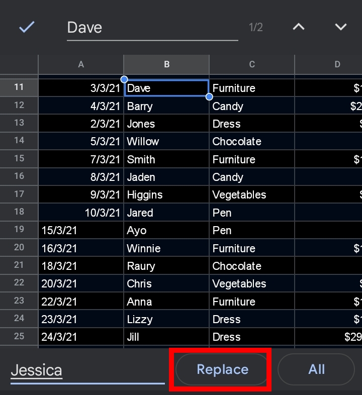
Step 6: Click Replace and each generated match is replaced with the new text. You can also replace the matching cells in a single go by clicking on Replace All.
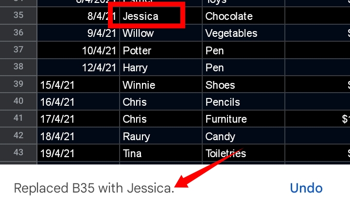
This method isn’t the best due to its limited features and functions. But in the absence of a computer or desktop, it is the best option if the task needs to be performed urgently.
How To Search in Google Sheets Using a Keyboard Shortcut.
Shortcuts make work easy as it can be done in less than a minute. Many features in Google Sheets can be accessed by shortcuts, search inclusive.
To easily access the Find and Replace feature, use the Ctrl key + H shortcut. This shortcut is mostly specialized in finding and replacing words only in Google Sheets.
This shortcut can’t be generally used in other applications like the copy and paste shortcuts.
Another shortcut used is the Ctrl key + F shortcut. This shortcut solely finds the entered text. It provides a textbox where the search key or text is entered.
The generated matches can be shuffled through and viewed individually by the use of the upward and downward arrows close to the search textbox.
How To Search All Tabs in Google Sheets.
In a case where you only want to find matches and don’t want to replace the matching texts, the Find and replace feature can also be used.
Step 1: Navigate your way to the toolbar and click on the Edit option on the toolbar.
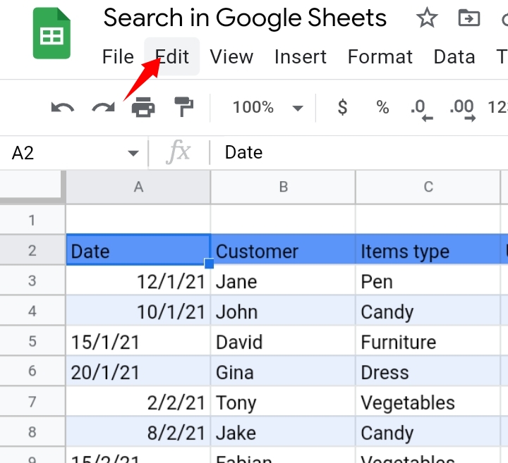
Step 3: From the drop-down list produced, select Find and Replace. Alternatively, you can directly use the keyboard shortcut, Ctrl key + H(Windows OS) or Command key + H(Mac OS) to open the Find and Replace tab.

Step 4: In the textbox directly beside Find, input the text string we want to search for. In this case, it is Smith.
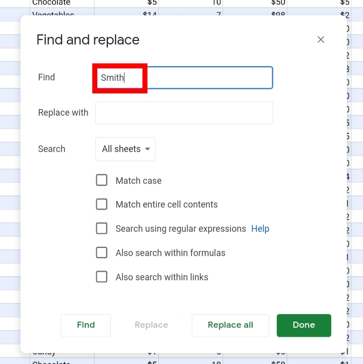
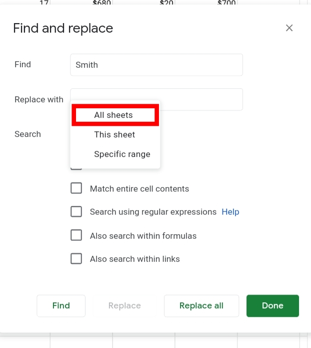
Step 6: Under search, click on the drop-down arrow here. Click on All Sheets.
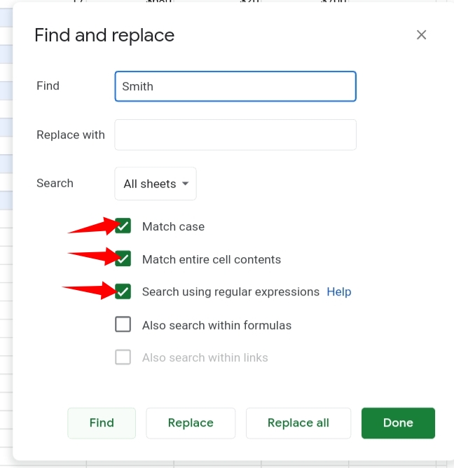
Step 7: There are five tick boxes with options. Select the first three options which are Match Case, Match Entire Cell Contents and Search using regular expression.
Step 8: Click on Find.
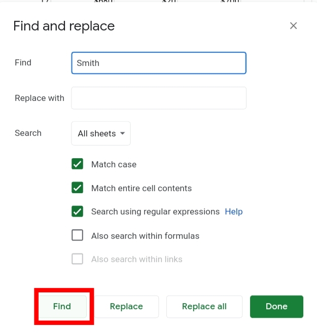
Step 9: The Find feature locates the matching cell but doesn’t replace the cell’s contents.
Final Thoughts.
This feature is a very helpful one. It helps to detect and replace duplicates of values in your dataset. I hope you can put this feature into good use in your entry experience with Google Sheets.
Now you know How To Search In Google Sheets. I hope you found this guide beneficial.


