In a case where you are constantly adding data and new values to a worksheet, you may want to know what the last value entered is to avoid repeating an entered value twice or multiple times.
Checking manually by scrolling down isn’t an option, because the human eye is prone to mistakes and cannot see and analyze multiple data at once.
Lucky for you, Google Sheets has just the trick to performing this task.
In this short guide, we are going to discuss and show you how to get the last value (both text and numerical values) in a column in Google Sheets with the use of a formula.
How To Get the Last Numerical Value When You Have Only Numbers.
In case you have only numbers in the column and you want to find the last value here, you would use the formula below.
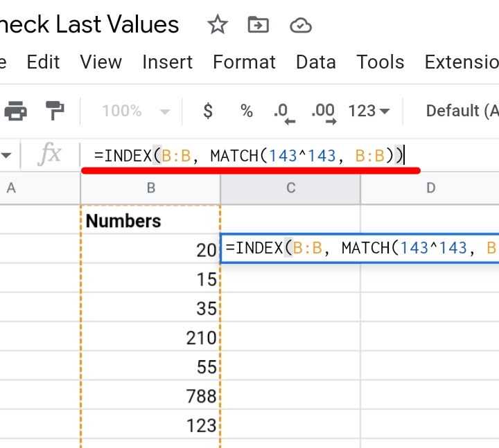
=INDEX(column range, MATCH(143^143, column range))
Step 1: Enter the formula =INDEX(B:B, MATCH(143^143, B:B)) into a cell where you want the returned value displayed.
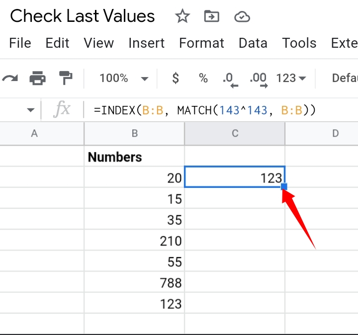
Step 2: Hit the Enter key on your keyboard and the last numeric value in the worksheet is returned.
How Does This Formula Work?
Notice that the formula is the combination of the INDEX and MATCH functions. The pair make a dynamic and accurate search function. In this case, the MATCH function locates the cell with the last numerical value in the selected column.
This implies that if there are five numbers in a column, the MATCH function would return a value of 5. Note that the function excludes empty cells if there are any in the selected column.
We are going to break down the formula to get a better understanding. The MATCH formula part is MATCH(143^143, B:B).
Starting with the first parameter in the MATCH formula, 143^143. This value is what the MATCH function would be searching for in the selected column range.
The second parameter, B:B is the column range where the MATCH function would search for the first parameter. The entire column is selected because we want to find the last value in the column.
So basically, the formula takes the lookup value which is 143^143 and searches all through the column to the end of the column for this value.
Since the value won’t be present in the column, it returns the last numerical value found in the column.
In the sample worksheet used, the MATCH function returns a value of 10 which is where the last value is.
The INDEX function simply extracts the actual value in the returned position which is 123.
How To Get The Last Text Value in A Column.
As the title implies, we would discuss how to find the last text value in a column with text values. Here, we have some names in column B.
So we quickly want to find the last name in the column. To do this, we need to use the formula and the steps below.
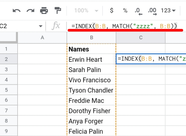
=INDEX(B:B, MATCH(“zzzz”, B:B))
Step 1: Enter the formula =INDEX(B:B, MATCH(“zzzz”, B:B)) into a cell where you want the returned value displayed.
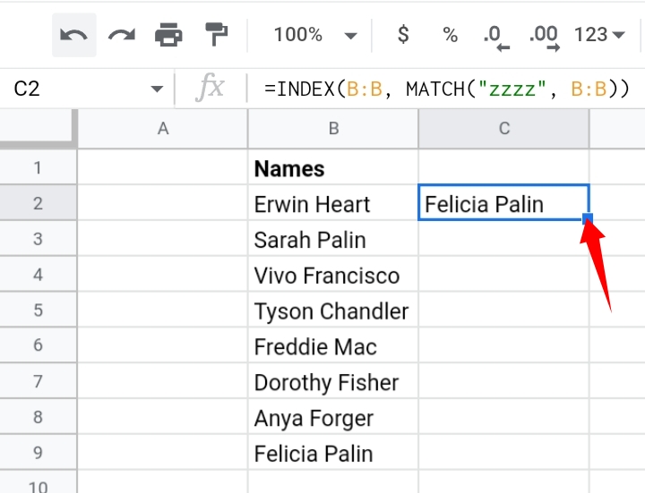
Step 2: Hit the Enter key on your keyboard and the last text value in the worksheet is returned.
How Does This Formula Work?
We are going to break down the formula into two parts. The MATCH formula part is MATCH(“zzzz”, B:B).
In this case, the “zzzz” statement acts as the search key. Since Z is the last letter of the alphabet, the MATCH function would search for the “zzzz” statement.
The “zzzz” statement is not going to be included in the selected column range so the MATCH function would return the last text value in the column since it was unable to find an exact match to “zzzz”.
Then, the INDEX function takes the returned position and returns the text value with the same position.
How To Get the Last Value in a Column With Both Text and Numerical Values
Now that we know how to get the last text and numerical values in a column, what do we do when the column has both values in a single column?
This is done by combining the formulas used previously and checking the location of the last cell which has the numeric and text value and returns the higher position.
The formula used is
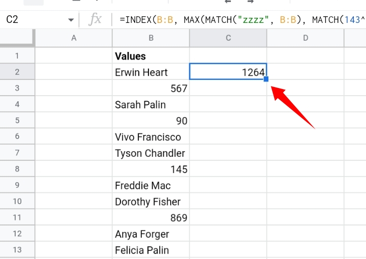
=INDEX(B:B, MAX(MATCH(“zzzz”, B:B), MATCH(143^143, B:B))).
Step 1: Enter the formula =INDEX(B:B, MAX(MATCH(“zzzz”, B:B), MATCH(143^143, B:B))) into a cell where you want the returned values displayed.
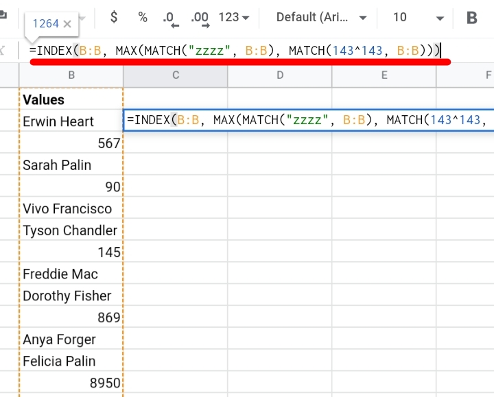
Step 2: Hit the Enter key on your keyboard and the last value in the worksheet is returned.
How Does This Formula Work?
The formula syntax deals with both the number and text values because the two formulas are combined as one.
The MATCH formulas are going to return a number that specifies the cells with the last number and last text string.
Then the MAX function compares the two numbers and extracts the bigger value and the INDEX function returns the value.
How To Use the INDEX and COUNTA Functions to Get the Last Value.
This method can be used when the selected range doesn’t have blank cells. If blank cells are in the column, the returned value would be affected and a wrong value would be returned.
The formula used takes the syntax below.
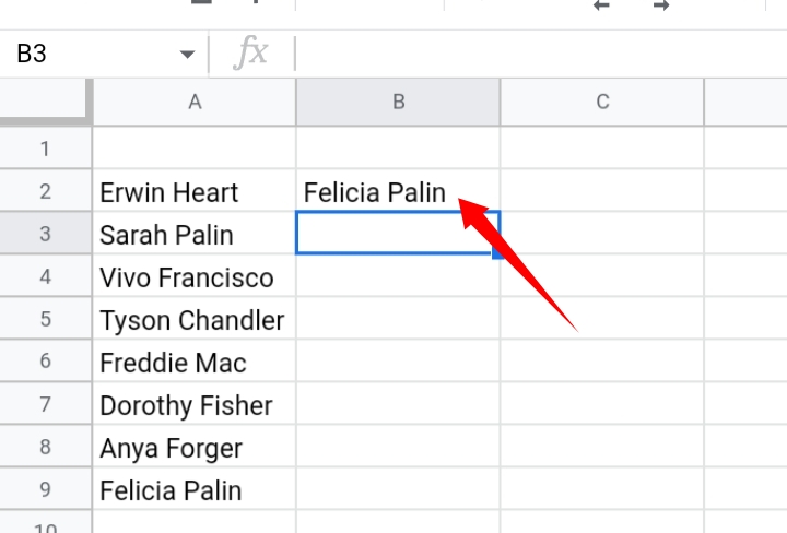
=INDEX(RANGE, COUNTA(RANGE))
Step 1: Enter the formula, =INDEX(A2:A, COUNTA(A2:A)) into the cell where you want the results returned.
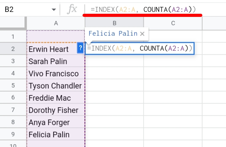
Step 2: Hit the Enter key and the last value is returned into the cell.
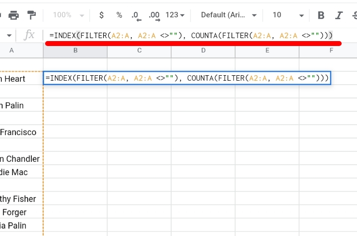
In a case where you have empty cells in the column, we’ll add the FILTER function to the previous formula. That is,
=INDEX(FILTER(column range, column range<>”), COUNTA(FILTER(column range, column range <>”))).
It is done in the following steps.
Step 1: Enter the formula
=INDEX(FILTER(A2:A, A2:A<>””), COUNTA(FILTER(A2:A, A2:A<>””))).
Step 2: Hit the Enter key and the last value in the column is returned.
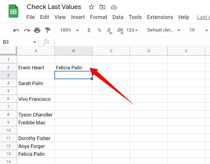
This formula is very suitable if you have blank cells in your selected column.
Final Thoughts
Now that we have covered this tutorial, I hope these formulas come in useful for you.
Now you know How To Get The Last Value In A Column In Google Sheets. Thanks for reading.


