How to Get Dynamic Range in Charts in Google Sheets [2022]

Do you ever get worried about the chart inserted on your worksheet when you need to add an extra cell or column to your dataset? A dynamic cell range is what your document needs.

In this tutorial, we are going to learn how to get dynamic range in charts in Google sheets. You can easily do that within a few minutes. So, let’s go.

What is a Dynamic Range?

A dynamic range is a range of cells and columns with added cells which changes the cell range and causes automatic adjustments to the chart. It also aids interactivity between the data in two or more cells in the worksheet.

How To Get a Dynamic Range in Charts in Google Sheets.

This is done by selecting the empty cells and columns and adding them to the old range. The dynamic range identifies the new cell and adds the data into the chart area, which causes the chart features to decrease as the chart area increases. 

Note that if an empty cell or column is added, the chart size won’t be affected.

How to Prepare a Drop Down Menu for A Chart.

Preparing a drop-down menu is the first step to getting a dynamic range for your chart in Google Sheets. This subtopic is divided into four categories which we would disseminate into steps and procedures.

Sample Data and Data Validation.

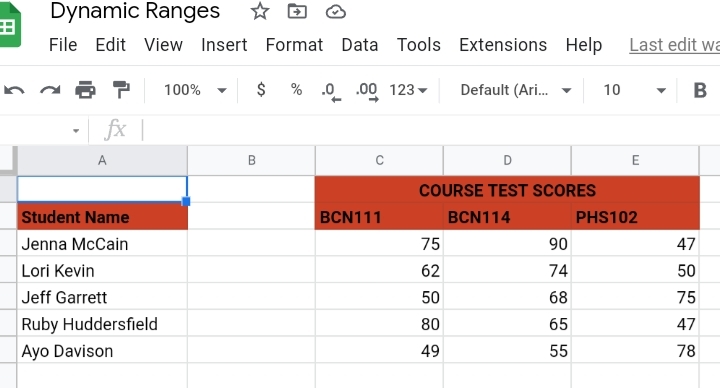
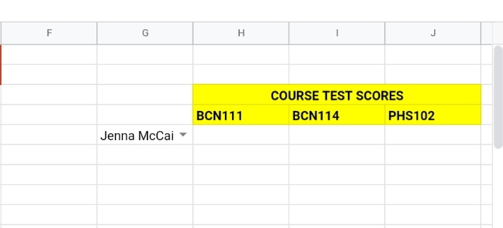
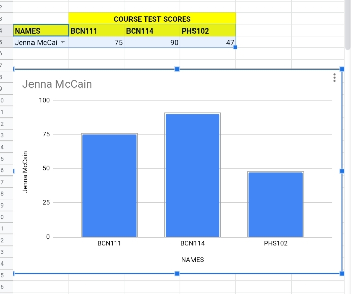
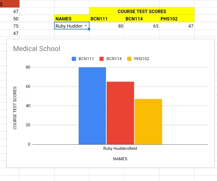
In the sample worksheet, we have a list of college students and their grades in different courses in Medical School. We want to get a dynamic range to create a dynamic chart which displays the relationship between the students and their scores.

 To achieve this, we need to create a data validation for the dataset.

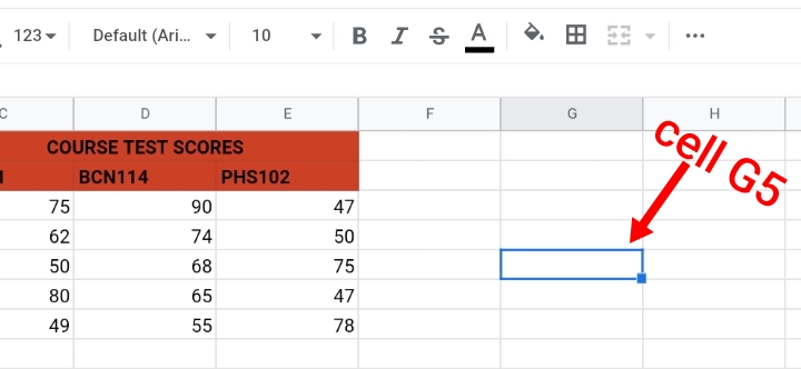
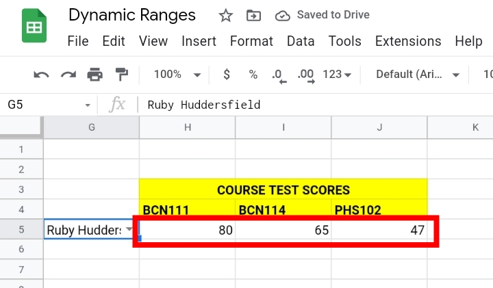
Step 1: Select any random cell on the worksheet where you want the validated data displayed. Note that you can’t use any cell that contains data for the raw data. So we selected cell G5.

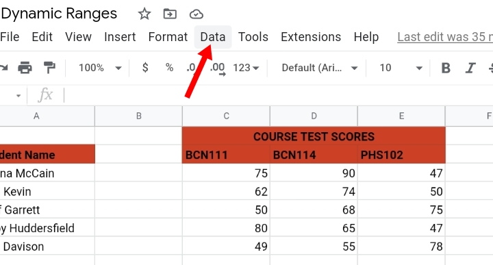
Step 2: Click on the Data icon on the toolbar.

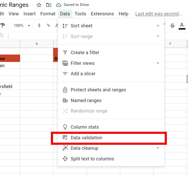
Step 3: From the drop-down menu produced, select Data Validation.

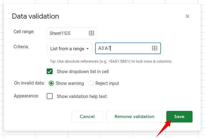
Step 4: A pop-up is shown on the worksheet. In the text box next to List from range, select the range of names of the students.

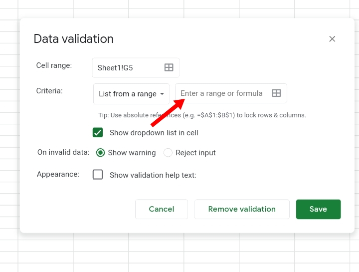
Step 5: Click Save here.

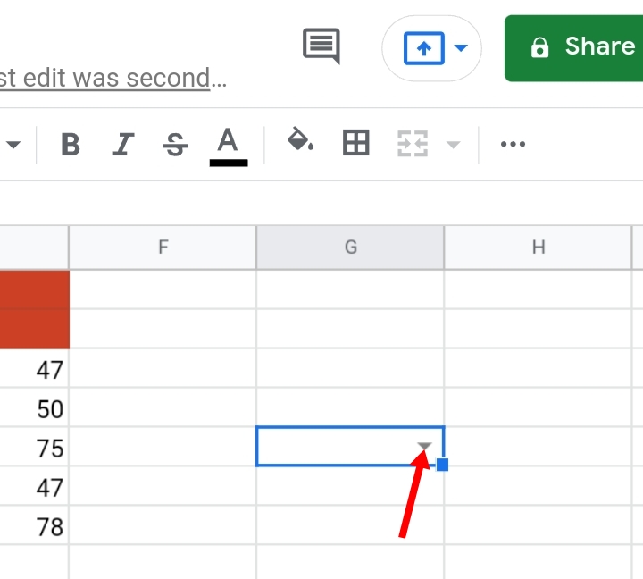
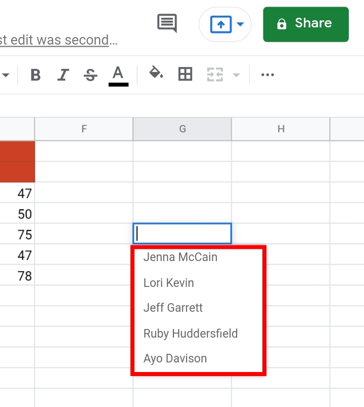
Step 6: In cell G5, a dropdown arrow is placed there, click on the arrow and the list of the college students is produced.

Formula For Drop Down Menu to Get a Dynamic Range In Charts in Google Sheets.

Now the first stage is completed, but a dynamic range hasn’t been created yet. This is where we employ the VLOOKUP formula to extract the matching scores of the respective college students from the original dataset. 

In the worksheet below, we have included the headers of the new data in their columns. Each header represents the courses studied by the students.

The VLOOKUP searches the actual dataset for matching data which is pasted into the columns in the new data. The formula used takes the syntax below.

=VLOOKUP(search key, range, index, [is_sorted])

Formula Explanation.

From the data in cell A3 to cell E7, we would analyze the parameters of the formula and the values substituted in the formula.

• Search key – This is a sample data that the VLOOKUP function takes as a search key to extract matching data and paste them into the new dataset. In this example, we selected the search key as G5.
• Range – This is the entire range of cells and columns of all students and their scores in the actual dataset. The range is inputted as A3:E7.
• Index – This is the index number of the columns which contain the scores. Columns A, B, C, D, and E are denoted as 1, 2, 3, 4, and 5 respectively. This also applies to other columns in the worksheet, as the alphabets increase, their index number also increases. Since we need to extract the scores of Jenna’s math course in column C, the index number is 3.
• Is Sorted – This is a factor added into the formula where the VLOOKUP searches for data if they are either true or false.

By substituting the values into the basic formula, we have

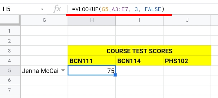
=VLOOKUP(G5, A3:E7, 3, [FALSE])

Step 1: Input the formula into cell H5.

Step 2: Press Enter on the keyboard and Jenna’s BCN111 test score is displayed.

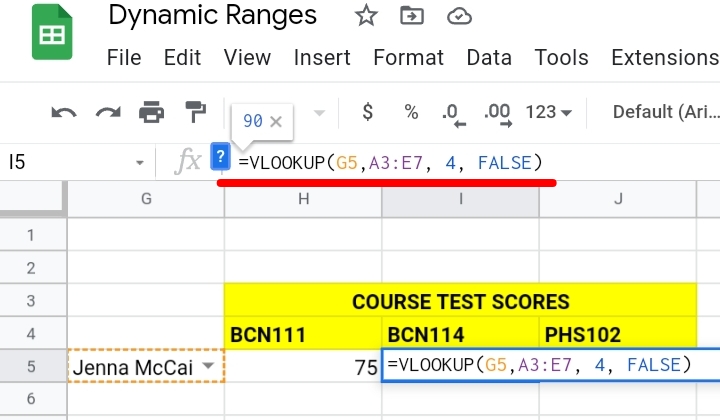
Step 3: Copy the formula and paste it into cell I5, but change the index number from 3 to 4, because we want to look up Jenna’s BCN114 test scores now.

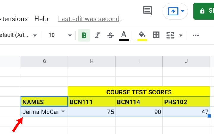
Repeat the steps for the last column too. A dynamic range has been created now.

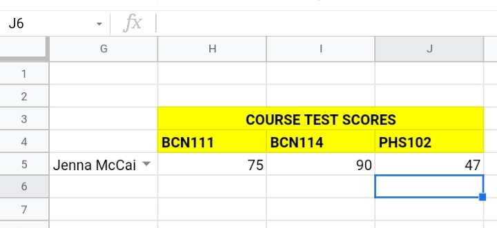
To prove this, by clicking on the drop-down arrow and selecting another student’s name, the test scores automatically change in correspondence with the student’s name.

Creating a Dynamic Range Chart.

Since we have a dynamic range created, we want to create a chart to illustrate the changes between the test scores and students’ names.

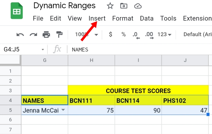
Step 1: Select the cell range of the new dataset.

Step 2: Click on Insert on the toolbar.

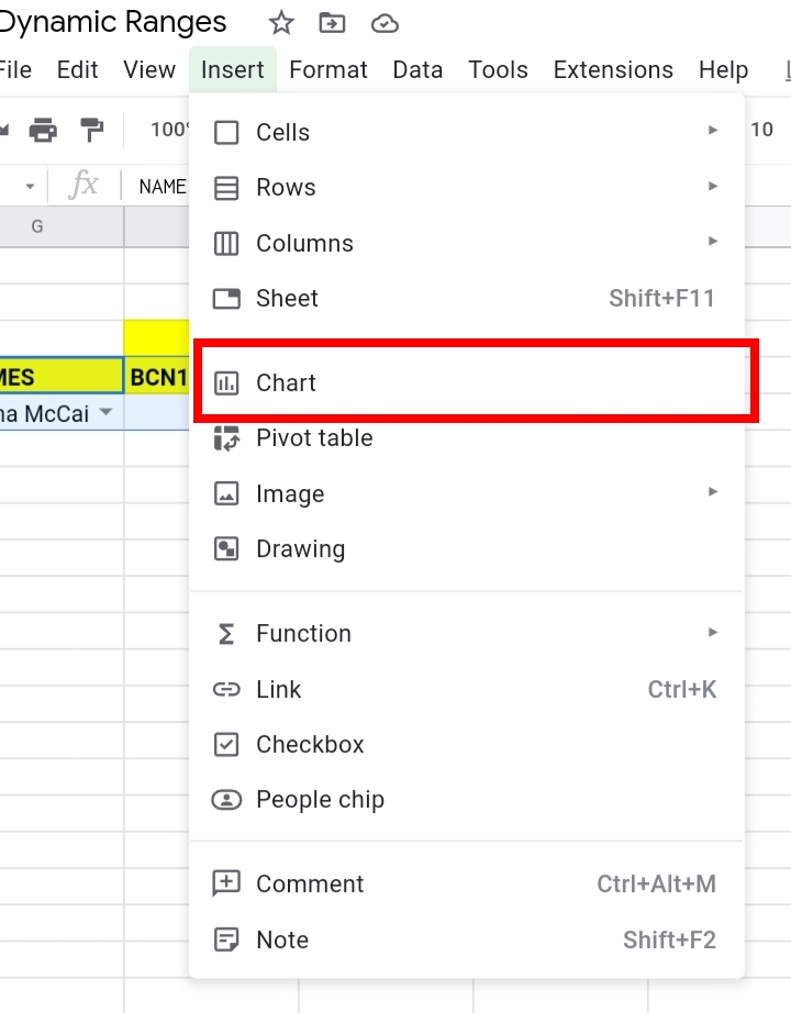
Step 3: From the drop-down menu produced, select Chart.

Step 4: Google sheets guesses what type of chart you want to use and produces a column chart. If you were given a different chart or you need a different chart, you can click on the three dots on the top right corner and click edit chart.

A tab is opened, under the Setup tab, select Chart type and select the chart of your choice.

Settings Under the DATA tab.

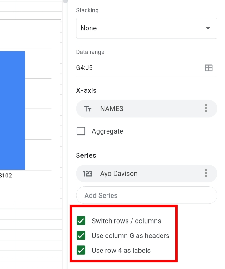
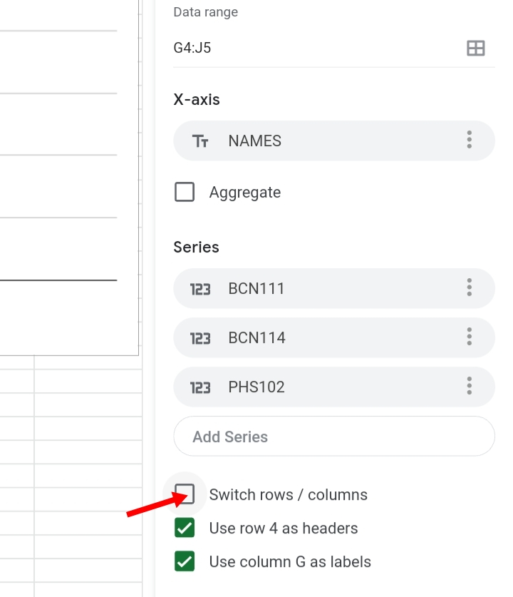
Here, we want to edit the bar chart by using the data tab. By clicking on the three dots on your chart, open your chart editor.

1. Under the Setup category, click on Chart type here.
2. Select Column Chart.
3. There are three ticked options stated here. Uncheck the Switch rows and columns.
4. The remaining options would be changed to use as headers and column G as labels.

Settings under the Customize tab:

 Under the Customize tab,

1. Select the Horizontal Axis and treat labels as text.
2. The chart automatically changes and the blank spaces in between the bars on the column bar chart are removed.

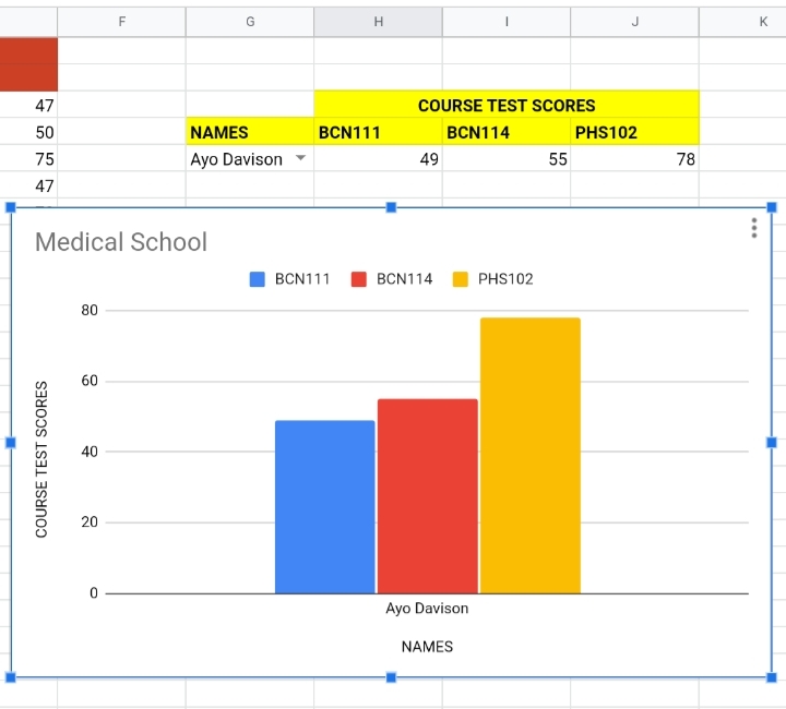
Now by selecting a different name, as the scores change, the bar chart changes accordingly.

Final Thoughts

This helps to prevent errors and automatically adjusts any extra cell or column to your chart and also helps to visualize any aspect of your data with ease. I hope you liked this tutorial. Thanks for reading.