When you want to perform a lookup task on your worksheet, the VLOOKUP and HLOOKUP functions are mostly employed. But what if I told you that there’s a better way of performing lookup tasks on your worksheet.
This technique is executed using the INDEX and MATCH functions, nested together into a single formula. Today we will show How To Use INDEX-MATCH Functions In Google Sheets. Before we delve into this topic, let’s discuss the INDEX and MATCH functions individually.
The INDEX function
This function returns the value located in the specified index. It also extracts the contents in a selected cell or cell range. That is, it analyses the selected cell, the given row index and a column index then returns the data in the selected row and column. The INDEX function takes the syntax below.
=INDEX(cell reference, [row], [column])
Where;
- Cell reference indicates the cell or cell ranges where we want to search.
- The row is the index number of a row within the specified cell range.
- The column is the column’s index number within the cell range which we want to search. This value is optional.
Using the sample worksheet below, we are going to explain how the INDEX function works. There are names of students in class A and their respective test scores.
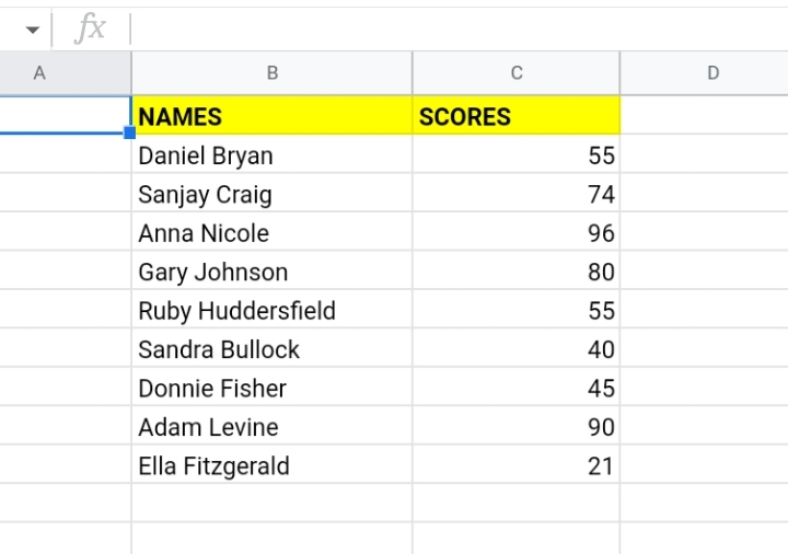
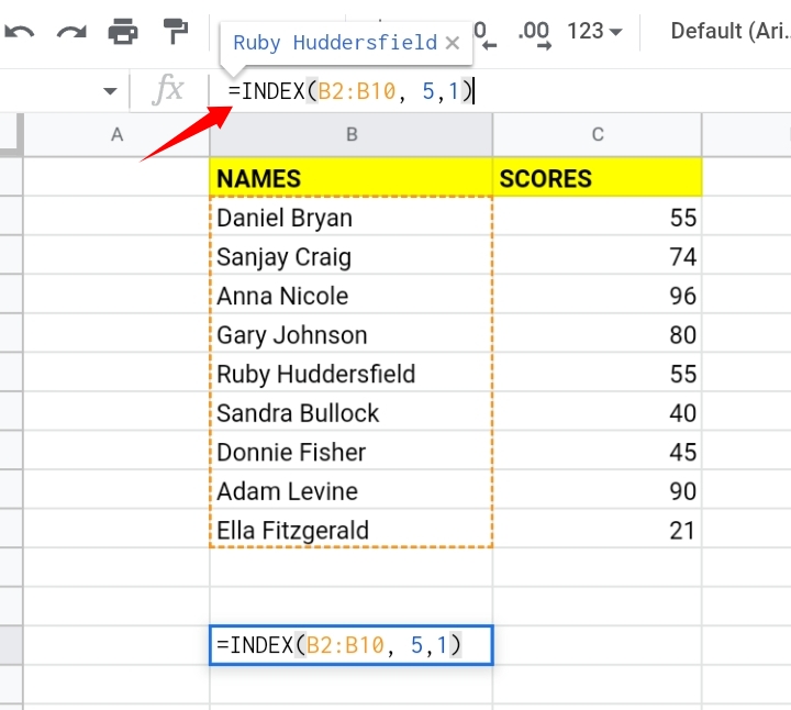
Now, we want to extract the fifth name in column B. The INDEX formula would be inputted like this.
=INDEX(B2:B10, 5, 2)
Step 1: Input the formula into an empty cell.
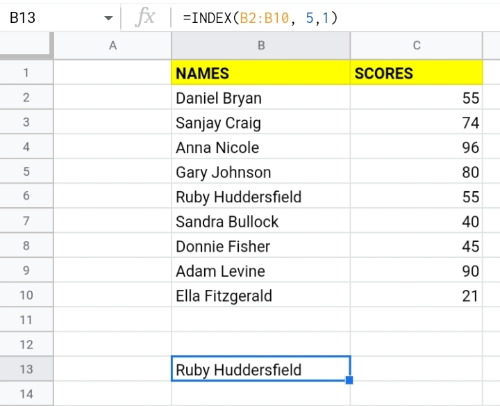
Step 2: Press the Enter key on your keyboard.
Step 3: The fifth name in column B is extracted and displayed in the empty cell.
The MATCH Function.
This function delivers the respective index of a value in a specific cell range. It analyses a cell range and returns the index of the item in the cell range. The MATCH function takes the syntax stated below.
=MATCH(search_key, range, search_type)
Where;
- The search key is the value we want to match in the cell range. It can be a text or number, cell reference or formula.
- The Cell range is where we want to search for the value corresponding with the search key.
- Search type is the kind of matching used. It is not compulsory to add this parameter to the formula. The search type is represented in numerical values. They are;
0: This specifies that the lookup is for a value that matches exactly with the search key.
1: This is the custom value. This value concludes the selected range is arranged in ascending order. This parameter extracts the largest value that is equal to or lesser than the search key.
-1: This value concludes that the selected range is arranged in descending order. This parameter extracts the smallest value equal to or greater than the search key.
Using the sample worksheet below, we are going to explain how the MATCH function operates. The worksheet contains the names of students in class A. Let’s say we want to know the position of “Adam Levine” in the worksheet. The formula used looks like this
=MATCH(‘Adam Levine’, B2:B10,0)
Step 1: Input the formula above into the empty cell.
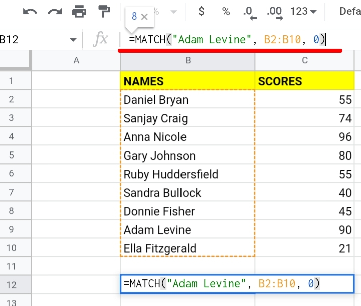
Step 2: Press the Enter key on the keyboard. A value of 8 is returned because the name is the sixth name on the worksheet, from cell B2, which is the starting cell.
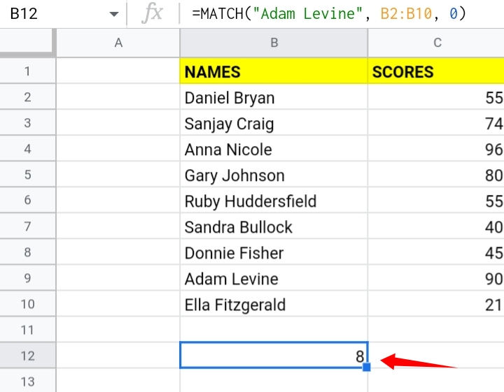
Note that the value returned is not a row number of the name but its position in the selected range.
Why use INDEX and MATCH Functions in Google Sheets?
Now that we’ve studied and understood their individual properties, we want to see what these two functions can do when nested into one formula. Separately, the INDEX and MATCH functions have very limited capabilities but we are going to combine them.
When nested as one, they can search for a value in a cell from the worksheet and return the results to another cell in the same data range.
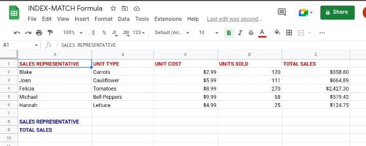
For instance, we have a dataset of the sales made in a Veggie store, all through the month. The worksheet consists of the names of the sales representatives, the goods sold, the units sold and the total sales made.
If we want to see the sales made by a salesman, the items sold or the unit costs, neither the INDEX nor MATCH functions can produce results individually. This is where their combination formula becomes helpful. In the next topic, we are going to discuss how to combine these functions as one.
How To Combine INDEX and MATCH functions in Google Sheets.
The combination formula takes the syntax below.
=INDEX(range2, MATCH(search_key, range1, 0))
Explanation of the Formula.
- Search_key is the item we are searching for in range1.
- Range1 is the cell range from which the INDEX function produces a value matching the position returned by the MATCH function.
- Range2 is the cell range from which the MATCH function produces a value matching the position returned by the INDEX function.
That is, the MATCH function helps to specify the index of the value returned to the INDEX function and vice versa.
Using the INDEX and MATCH Functions with Single Column References.
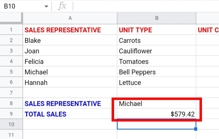
As stated earlier, the sample worksheet contains the names of sales representatives, units sold, the unit cost and the total sales made. At the bottom of the dataset, there’s a small table where we have the name of the sales representative and the total sales made.
The table is subject to change, so we cannot tag the name inputted as the absolute reference. Here, we are going to use the nested formula of the INDEX and MATCH functions. The formula used is inputted in the bottom table like this.
=INDEX(E2:E6, MATCH(B8, A2:A6,0))
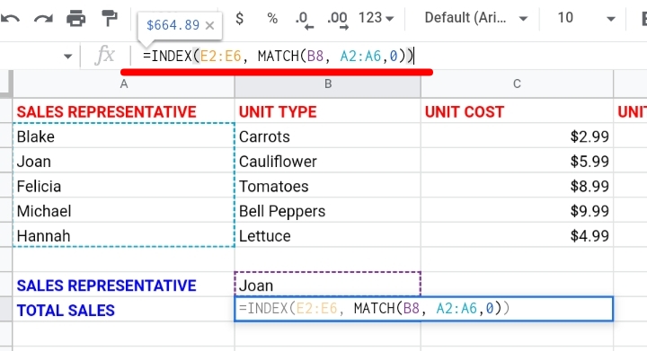
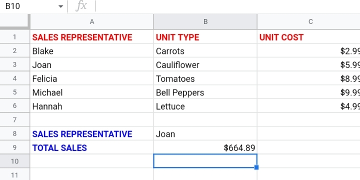
Press the Return key and the total sales made by Joan are returned to cell B9.
Explanation of the Formula.
Starting from the inner formula which Is MATCH(B8, A2:A6,0)
The MATCH function scans the range A2:A6 for the name in B8. Since Joan is the second name from the starting cell A2, the MATCH function returns the position as 2.
Next is the INDEX formula which is =INDEX(E2:E6). The formula searches for the name in the second position of the cell range E2:E6 and returns the total sales made by Joan.
Now, We changed the name in cell B8 from Joan to Michael. The table is dynamic, so the total sales for Michael also changed.
Using INDEX and MATCH Functions with Multiple Criteria.
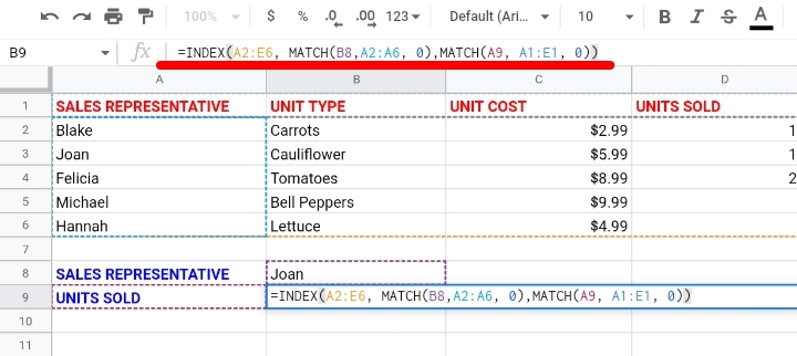
The INDEX-MATCH provides flexibility in your worksheet by gaining access to multiple columns at a time. In the sample worksheet used previously, let’s change the headers of the bottom table. That is A8 represents Sales Representative while A9 represents the units sold.
Now that we’ve added a different header, the table seems more dynamic. This means we need to evaluate multiple columns and the columns will depend on cell B9. This would be done by using the INDEX-MATCH function below.
=INDEX(A2:E6, MATCH(B8, A2:A6, 0), MATCH(A9, A1:E1, 0))
Here, there is a third parameter in the INDEX-MATCH formula. This parameter searches for the index of the selected header in the header row.
In the worksheet below, cell A9 contains “Units Sold”. This formula returns units sold that match the name in cell B8. If a name is entered in cell B8, the unit sold by the person is entered in cell B9.
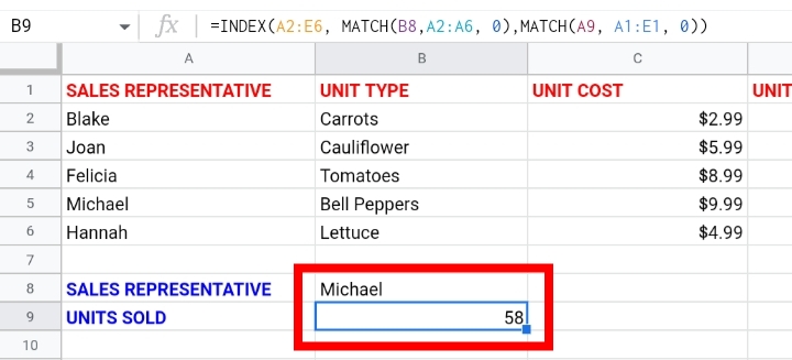
Even if the name is changed, the correct unit sales are returned in cell B9.
Explanation of the formula.
This formula has three parameters, we are going to break each one down to your understanding. We are going to start with the first MATCH function in the formula.
MATCH(B8, A2:A6,0).
The first MATCH function extracts the position of Joan’s name in the selected cell range. So it returns the index number of 2.
Next is the second MATCH function,
MATCH(A9, A1:E1, 0).
The second MATCH function scans the cell range A1:E1 for the value in cell A9 and extracts the position of the corresponding value. The text in cell A9 says “Units Sold”, the function finds the text as the third value from the starting cell A1 and it returns the index number 4.
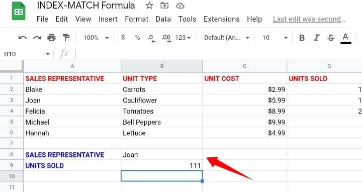
Lastly, the INDEX function =INDEX(A2:E6, MATCH(B8, A2:A6, 0), MATCH(A9, A1:E1, 0)).
The formula searches for the second position in the row and fourth position in the column in the cell range A2:E6 and returns the value of the index which is ‘111’. This is the unit sales made by Joan.
How To Use MATCH Formula in Google Sheets.
Here, we are going to see how to use the MATCH function vertically and horizontally on the worksheet.
Vertical Use of MATCH function in Google Sheets.
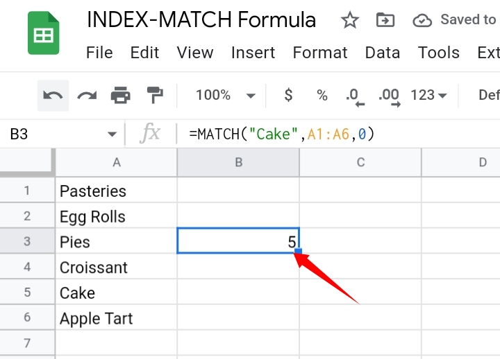
As stated previously, the MATCH function only returns the position of the item and not the exact value. In the sample worksheet, we want to see the exact position of “Cake” vertically. The formula used is
=MATCH(“Cake”, A2:A6,0)
Where Cake is the search key while A2:A6 is the search range and 0 implies that the data is unsorted.
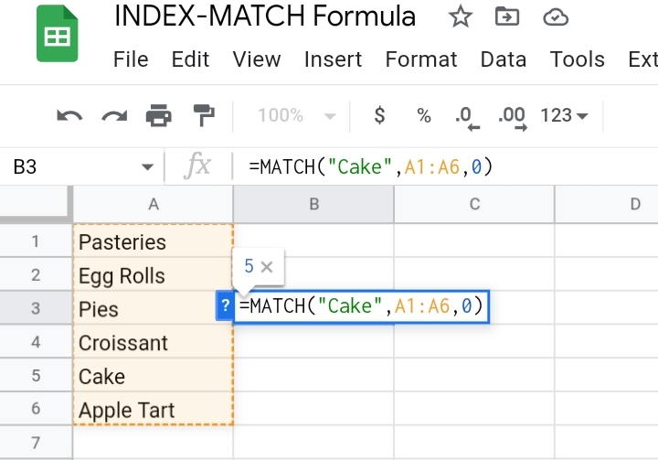
The formula returns the number 5.
Explanation.
Notice the selected range A2:A6, it is a single column. You can use a single column in a MATCH formula only whether it’s vertical or horizontal.
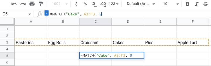
Horizontal Use of MATCH function in Google Sheets.
When you have a dataset and you want to use the MATCH function on a single row horizontally, the cell range would be the range of rows. The formula used is
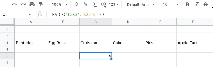
=MATCH(“Cake”, A3:F3, 0)
The MATCH function scans and extracts the exact position of “Cake” horizontally.
Why is Using INDEX and MATCH better than VLOOKUP?
The properties above can also be done with a VLOOKUP function but there are some aspects of the INDEX-MATCH formula that surpasses the VLOOKUP.
First of all, added columns or shifting existing cells and columns do not implicate the returned values of the INDEX-MATCH formula because it permits cell references. However, the VLOOKUP results get influenced by the moving or addition of new columns because it evaluates the column order only.
Secondly, the INDEX-MATCH formula permits the search on both the left and right sides of the columns while the VLOOKUP only permits the search on the left of the column. If you try to access the right of the search column, a #N/A error is returned.
Lastly, the INDEX-MATCH function is very flexible and dynamic especially when dealing with cell references compared to the VLOOKUP function.
Case Sensitive VLOOKUP With INDEX-MATCH in Google Sheets.
The INDEX-MATCH function is the best option when dealing with case sensitive data.
In the worksheet below, suppose some bottled sodas are sold in cartons and are also sold per piece. Hence there are two circumstances of the types of soda, with their prices per piece and per pack.
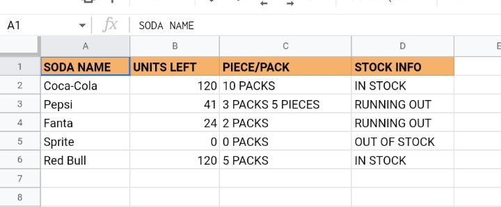
What if we want to extract the stock of each item? The VLOOKUP function isn’t suitable for this task because it always returns the first name found.
Here’s where we use the INDEX-MATCH function but an additional function is included which is the FIND function. The FIND function is a case sensitive function which makes it most suitable for this task.
The formula used takes the syntax below.
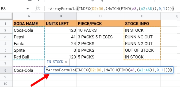
=ArrayFormula(INDEX(D2:D6, (MATCH(FIND( A8, A2:A6)), 0,1))))
The FIND function analyzes the Item Name column which is column A (A2:A6) for the text in cell A8(Coca-Cola). Once found, the formula tags the cell with the number 1.
Then, MATCH searches for the tag and gives the tag to the INDEX function. INDEX comes to the corresponding row in column C and extracts the stock info on the item.
Be sure to add the ArrayFormula at the start of the whole formula because, without it, the FIND function won’t search in array order.
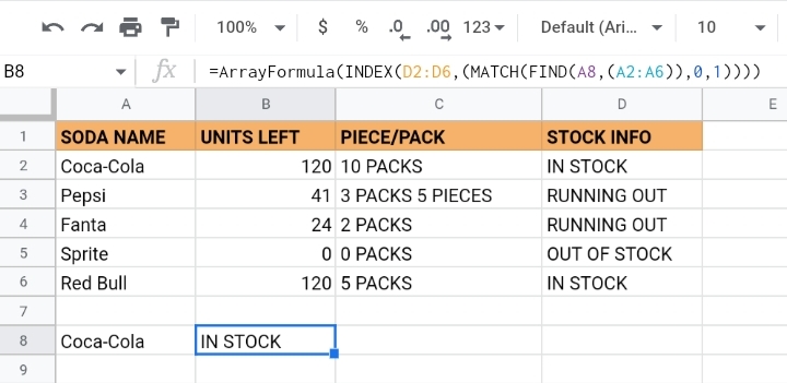
In the result cell, the stock info is extracted as seen below.
Final Thoughts
The INDEX-MATCH combination formula is a very dynamic and important way of searching and extracting important aspects of your data. Learn this formula properly to use it at its best.
Now you know How To Use INDEX-MATCH Functions In Google Sheets. I hope you found this guide helpful.


