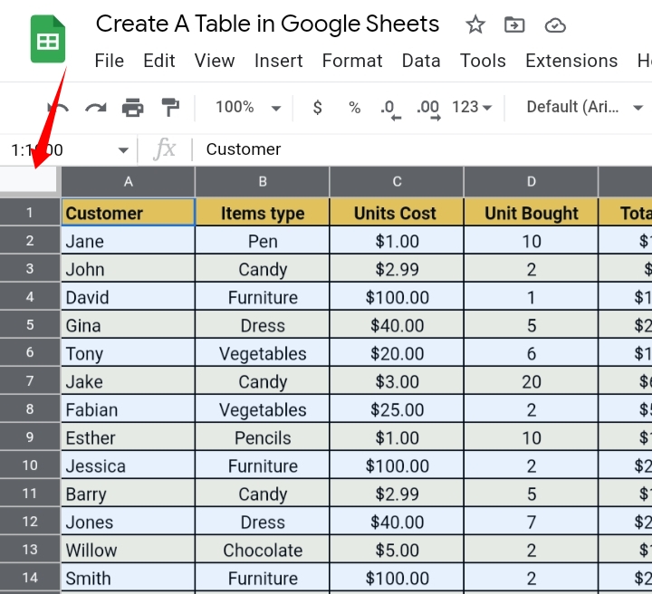
Entering data into your worksheet in a regular way may seem alright but what if you want to present your dataset in a tabular form to improve readability and comparisons between the values in the dataset.
Inserting a table into your worksheet is exactly what you need in this case. Unlike Microsoft Excel, there is no direct way or inbuilt feature to do this in Google Sheets.
In this how-to guide, we would discuss and learn How To Make A Table In Google Sheets by modifying your regular data into a tabular form.
How To Make A Table In Google Sheets With Formatting.
The major way of inserting a table into Google Sheets is by Formatting. All other methods are birthed from formatting.
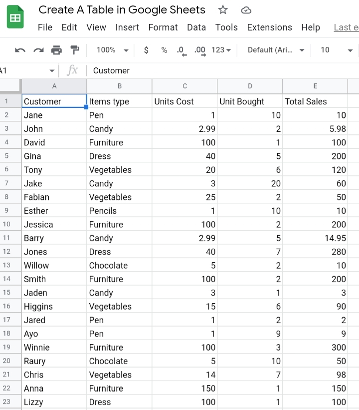
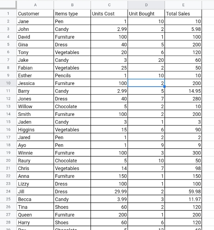
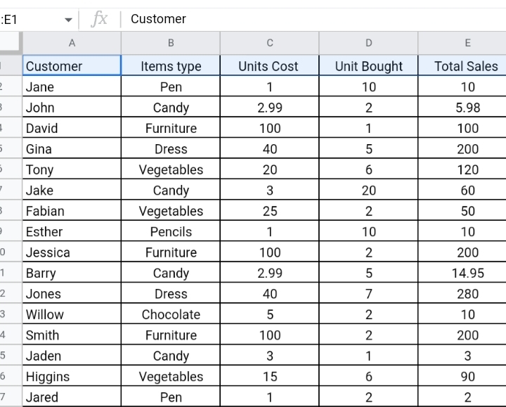
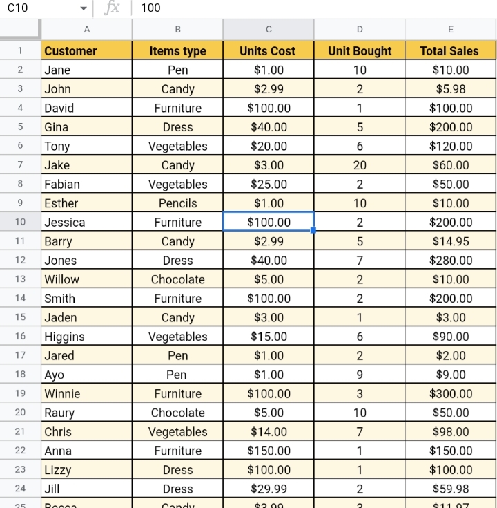
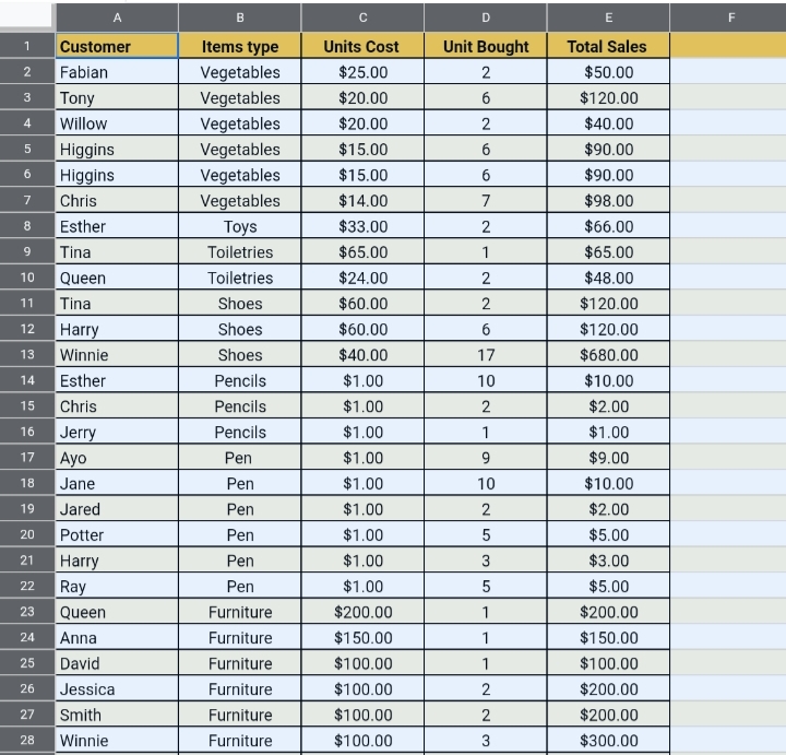
Using our regular old and boring worksheet below, we would modify it into one that is better looking and appealing to other viewers. I would show you all the available methods used to create a table.
Making A Table in Google Sheets by Applying Borderlines.
If you apply borderlines on the cells, it would produce the impression that the dataset is tabularized. This is done by following the steps below.
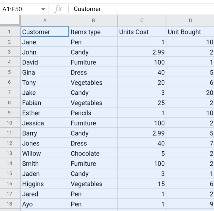
Step 1: Select or highlight the dataset you want in a table.
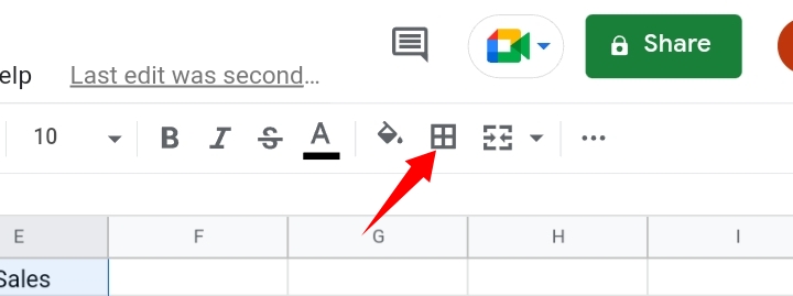
Step 2: Navigate your way to the toolbar and click on the border style icon.
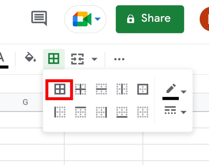
Step 3: Select the border style from the given options.
Step 4: You can see the data set’s new look. It looks more like a table now.
How To Insert A Table In Google Sheets By Aligning The Data.
Text Alignment in Google Sheets is a very useful feature. It helps to keep your entered values more organized and easy to read.
There are three known alignments in Google Sheets which are Left, Center/Middle and Right alignments.
In a custom setting, numerical and text values are aligned on the left and right sides of a cell respectively.
Here, we would use the centre alignment to create a table. This is done by following the steps below.
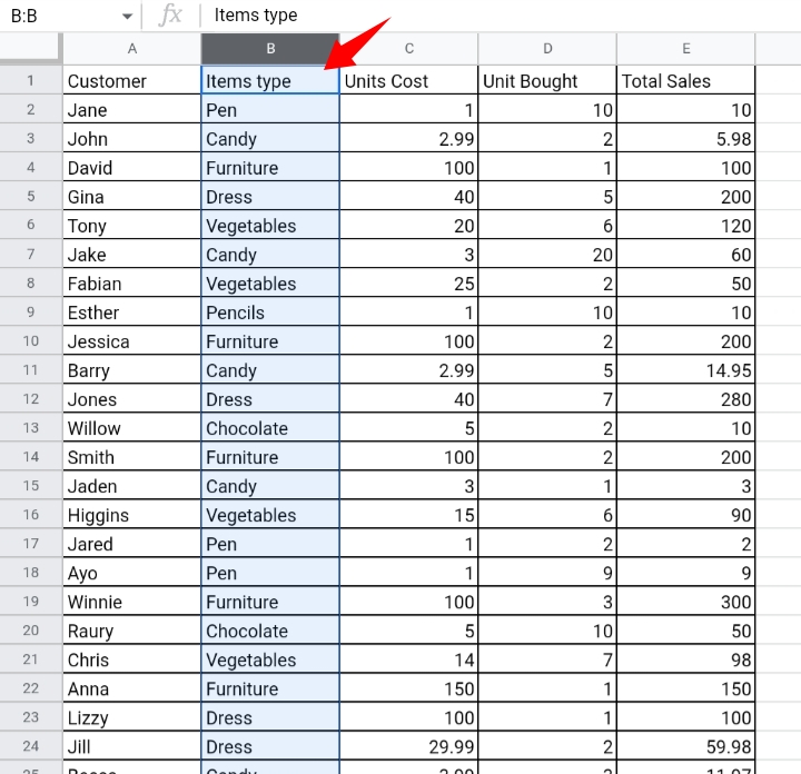
Step 1: Select the columns you want aligned. You may also want to align the headers of your dataset.
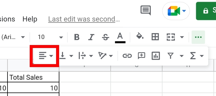
Step 2: Go to the toolbar and click on the Text Alignment icon.
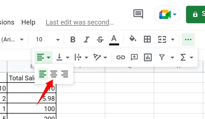
Step 3: Select the Middle or Centre Alignment icon.
Step 4: Now, the selected values are positioned in a centre alignment. This makes your worksheet look more presentable like a table.
How To Create A Table In Google Sheets With Coloured Or Bold Headers.
Most Google Sheets users are probably familiar with coloured headers in their worksheets but how do we use them to create a table?
By using the coloured headers, it emphasizes and describes what the worksheet is about.
If you open a worksheet with coloured headers, you would initially look at the headers because they are coloured and tend to gain more attention than the other contents in the worksheet.
To create a table with this method, you need to follow the steps below.
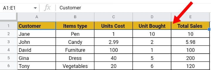
Step 1: Highlight the headers in the worksheet.
Step 2: Go to the toolbar and click on Bold. Alternatively, you can use the keyboard shortcut, Ctrl key + B(Windows OS) or Command + B(Mac OS) to add the bold format to the headers.

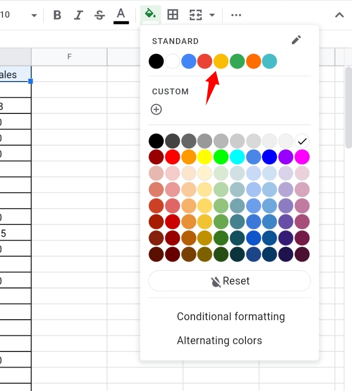
Step 3: Next, click on the Fill Color icon on the toolbar.

Step 4: A color panel is displayed. Here, you can select any color of your choice. In this case, we selected the color yellow.
Now, the headers of your worksheet won’t look so plain and simple but more like a colourful table.
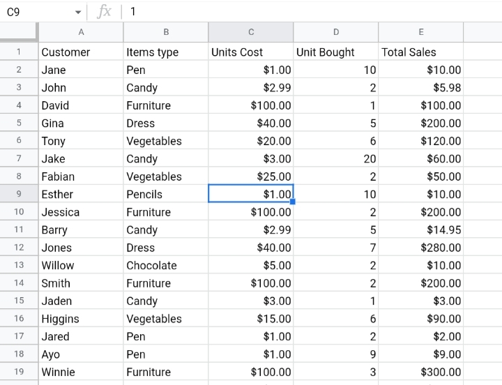
Format As Table In Google Sheets – The Numbers.
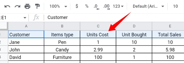
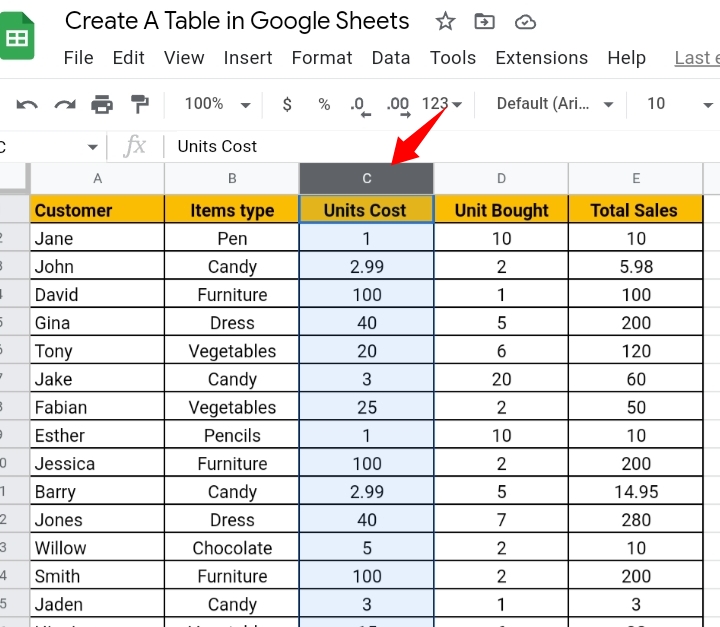
In a case where you have numbers in your worksheet like sales, budgets or costs, you may need to format them to make them look more like actual costs and more meaningful.
In this sample, we have some item budgets in dollars. We need to add the currency sign and format. To do this, we need to follow the steps below.
Step 1: Highlight or select the cells in the Units Cost column.
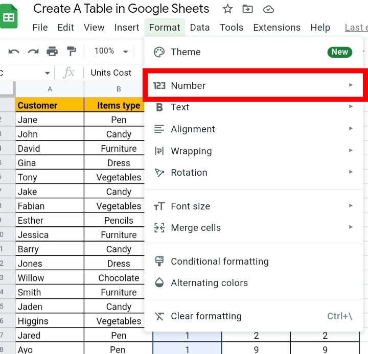
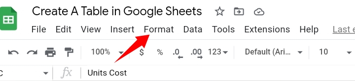
Step 2: Go to the toolbar and click on Format.

Step 3: Click on Number.
Step 4: From the drop-down list, select the Currency format.
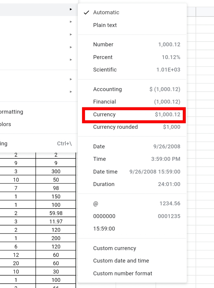
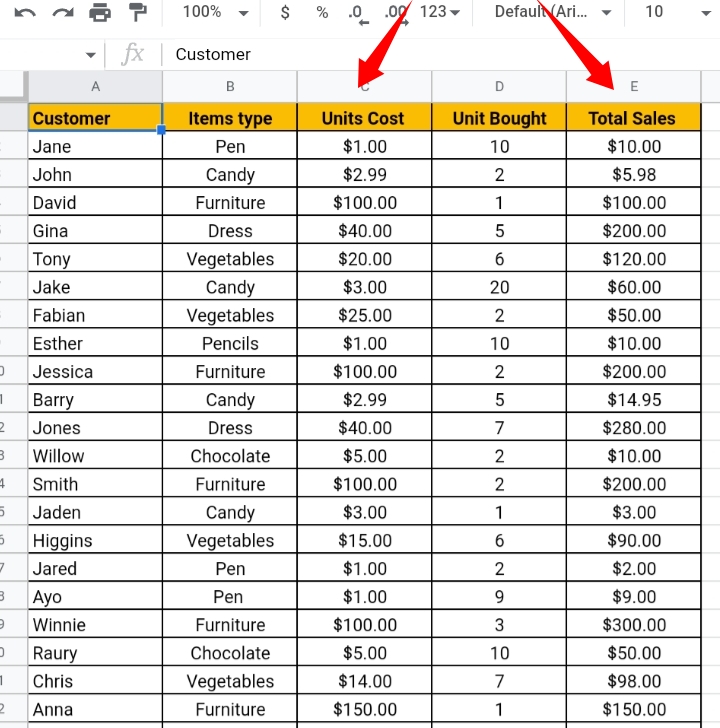
Step 5: Here, the currency symbol is added to the values. You can also round the values off by the thousand format and decimal places if the cost is also in cents.
Repeat this process for other columns with numerical values that need to be formatted.
Here’s what your table would look like.
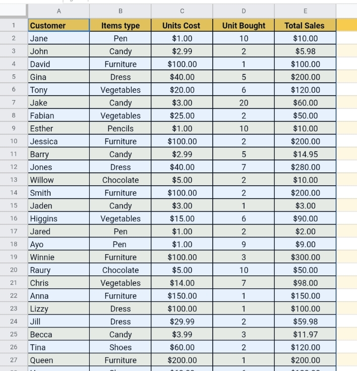
Advanced Google Sheets Table Formatting- Applying Alternate Colors To Rows.
Now let’s take a step further. In a case where you want to do more formatting to drastically improve your worksheet’s conciseness and readability, you would need to apply alternate colours to the cells.
To do this, you would need to take the steps below.
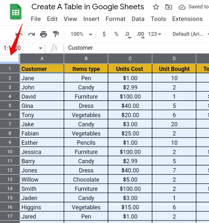
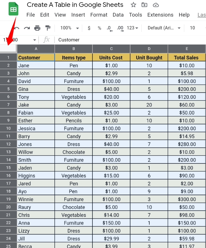
Step 1: Select all the cells and columns in the dataset by clicking on the grey box here.
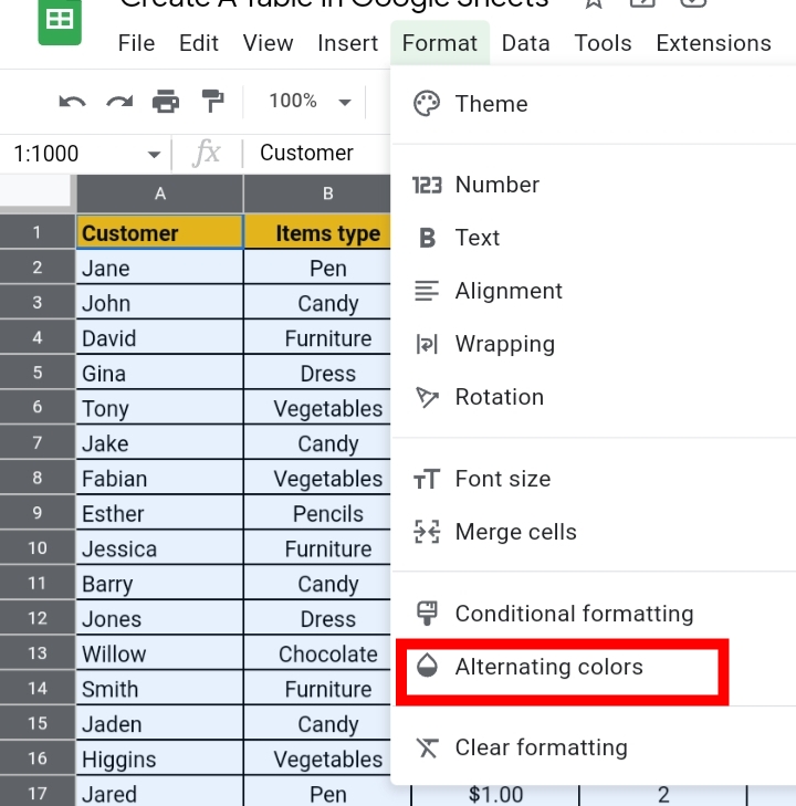
Step 2: Go to the toolbar and click on Format.

Step 3: Next, click on Alternating Colors.
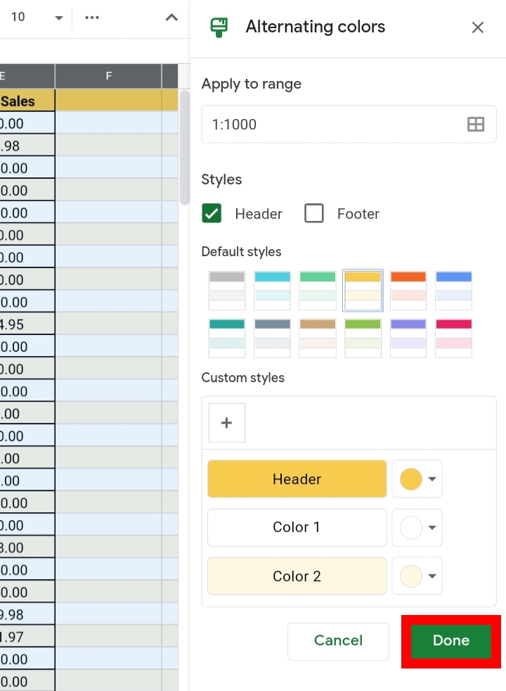
Step 4: The color of the cells turns into a lighter shade than the color of the header row. Also, the “Add Alternating Color” tab is opened at the right of the worksheet.
Step 5: In this tab, you can customize and change the colors of the header rows and rows in the worksheet.
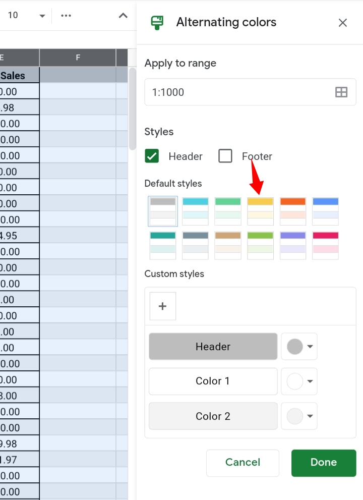
Step 6: Select a color and click Done.
Here’s how the table colours are like.
Advanced Google Sheets Format Table Ticks – Sort The Columns.
This helps to improve the reading flow and conciseness of your worksheet’s content especially when you’re working with large data with multiple columns and rows.
To do this, you would need the following steps.
Step 1: Select all the cells and columns in the dataset by clicking on the grey box here.
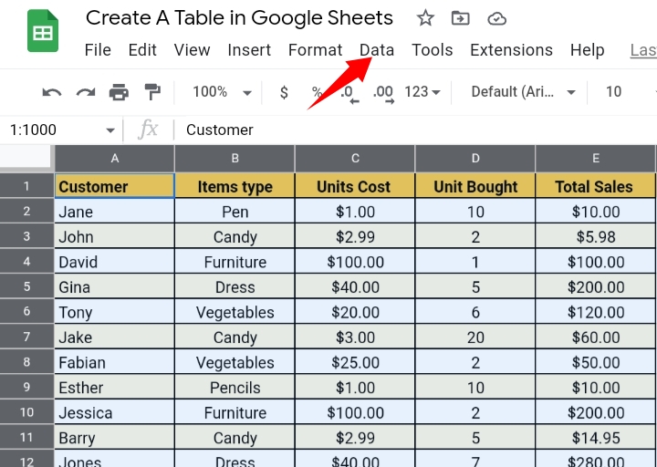
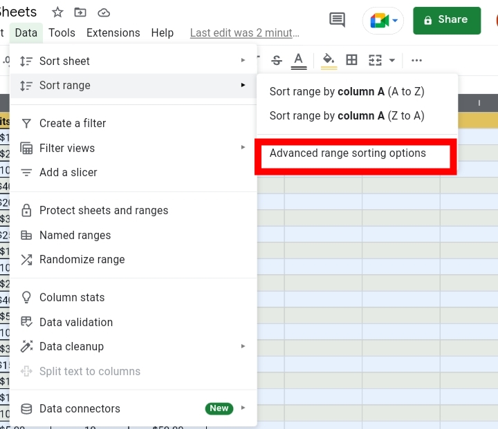
Step 2: Go to the toolbar and click on Data.
Step 3: From the drop-down menu, select Sort Range.
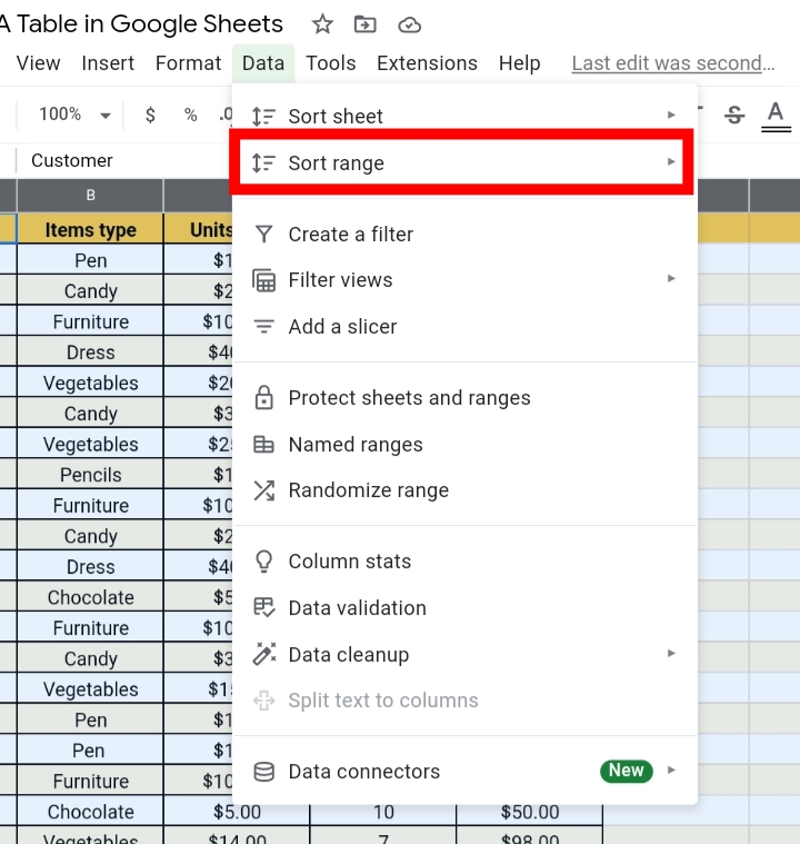
Step 4: Select Advanced Range Sorting Options here.
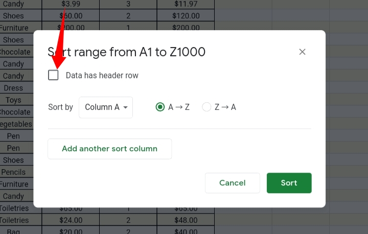
Step 5: The Sort tab is opened. Here, you can set how you want Google Sheets to sort your dataset.
Step 6: In the row section, check Data has headers.
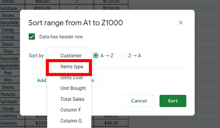
Step 7: In the Sort section, select Items Type.
Step 8: Click on Add Another Sort Column.
From the drop-down, select Unit Sales and set the order as Z to A. This order sorts the datasets in descending order.
Step 9: Click Sort. The dataset would be sorted according to the selected columns, that is by Items type and Units Cost.
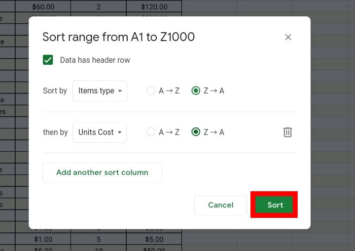
By sorting the columns, other viewers can easily see what item they require and the sales made on the particular item. Easy peasy!
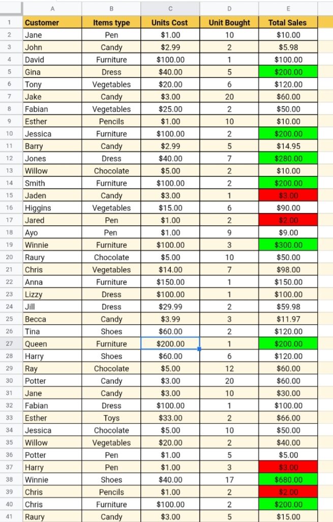
Advanced Google Sheets Format as Table Ticks – Highlight High and Low Values.
To speed up data analysis in your worksheet, you may highlight important values. In this sample, we would highlight the top five highest sales and lowest sales made.
To do this, we would use Conditional formatting by following the steps below.
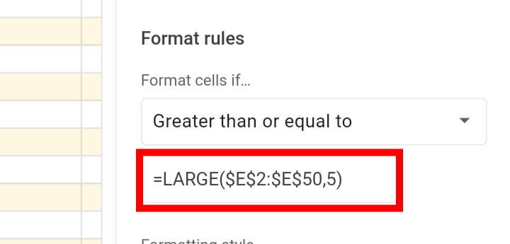
Step 1: Select the cell range containing the values you want to work with. In this case, we want to see the highest and lowest values so we selected range E1 to E50.
Step 2: Navigate your way to the toolbar and click on Format.
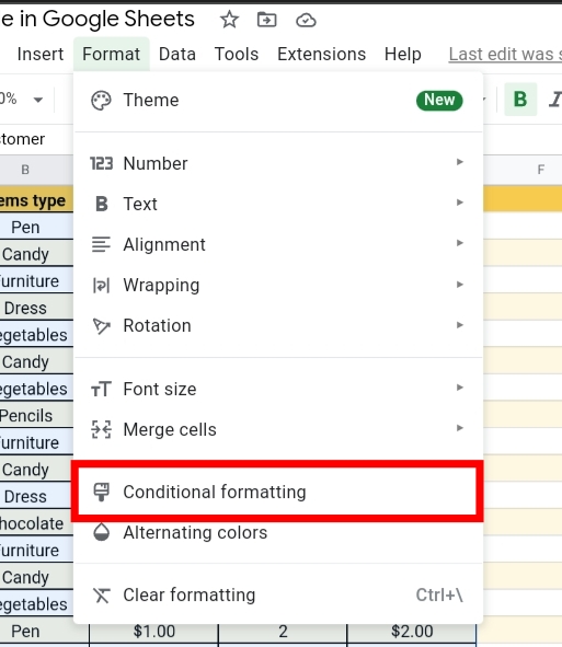
Step 3: From the list, select Conditional Formatting.
Step 4: The Conditional Format tab is opened at the right end of the worksheet.
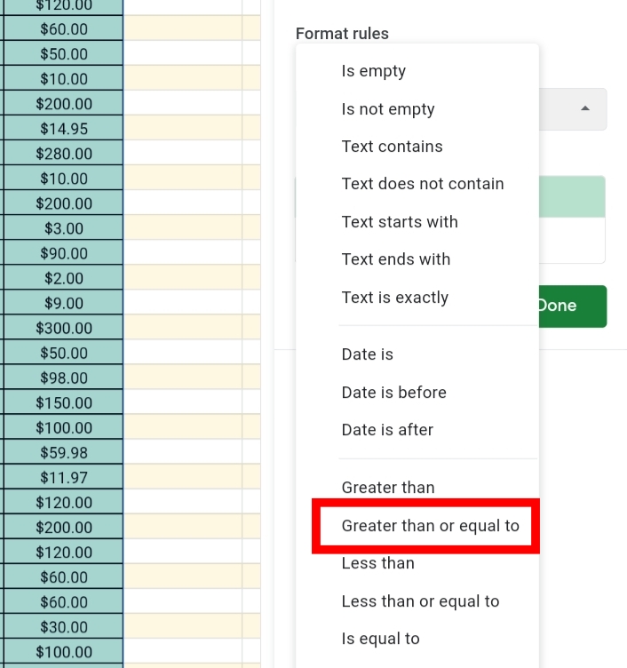
Step 5: Under the Format Cells If, select ‘Greater than or Equal to’ from the drop-down list provided.
Step 6: In the text box, enter the formula
=LARGE($E$2:$E$50, 5)
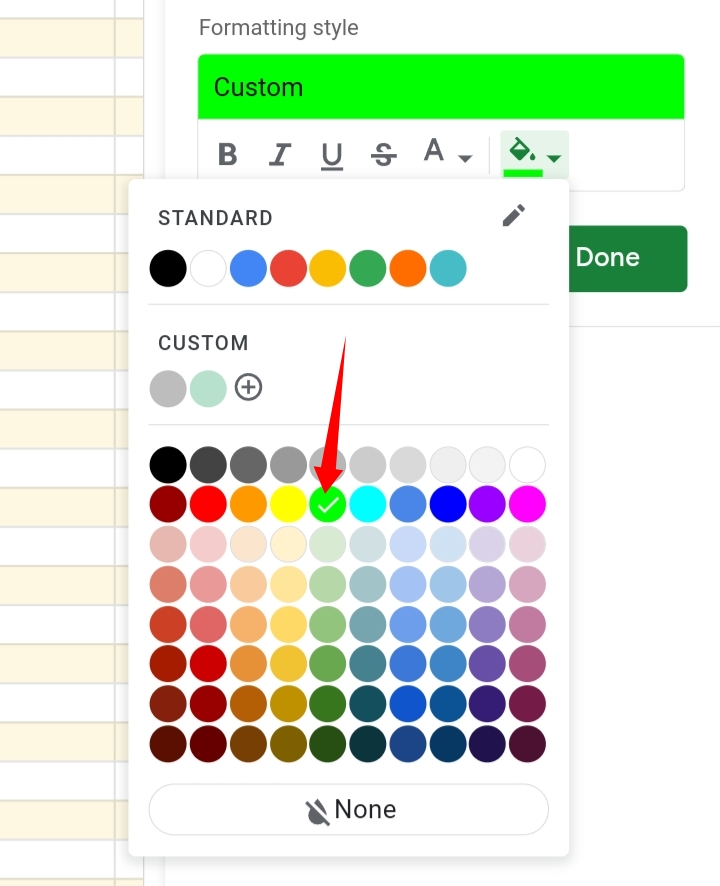
Step 7: You can customize how you want the highlight’s format to look. That’s if you don’t want to use the default format and colours. In this example, I selected green.
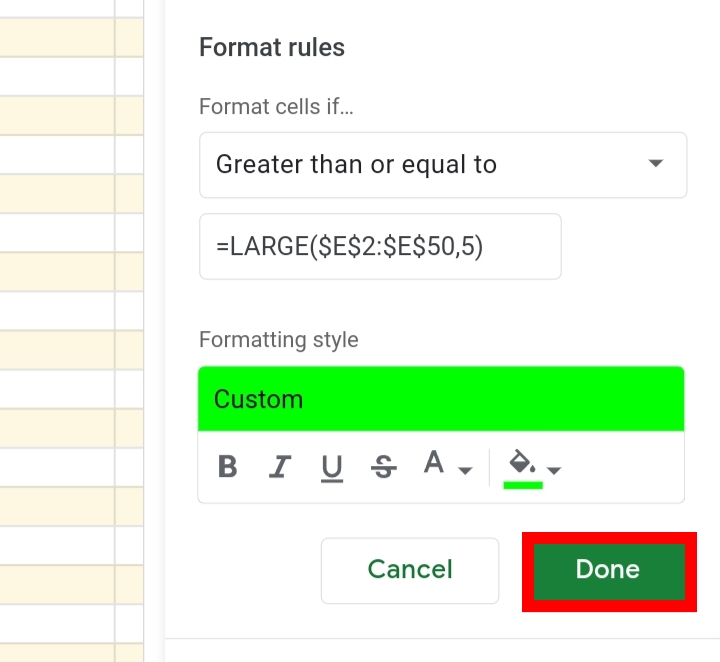
Step 8: Click Done. The steps listed above would highlight the highest sales.
To get the top five lowest sales, you would follow these steps below.
Step 1: Select the cell range of the dataset.
Step 2: Navigate your way to the toolbar and click on Format.

Step 3: From the list, select Conditional Formatting.

Step 4: The Conditional Format tab is opened at the right end of the worksheet.
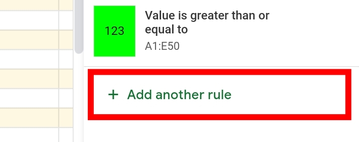
Step 5: You would add another rule.
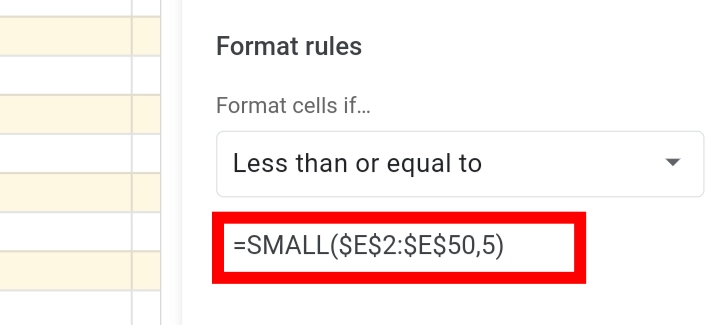
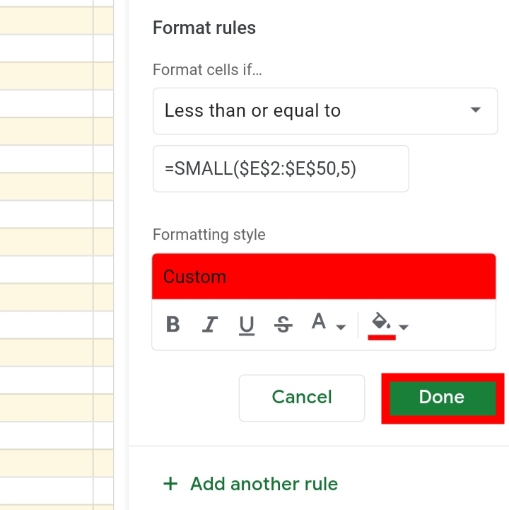
Step 6: Under the Format Cells If, select ‘Less than or Equal to’ from the drop-down list provided.
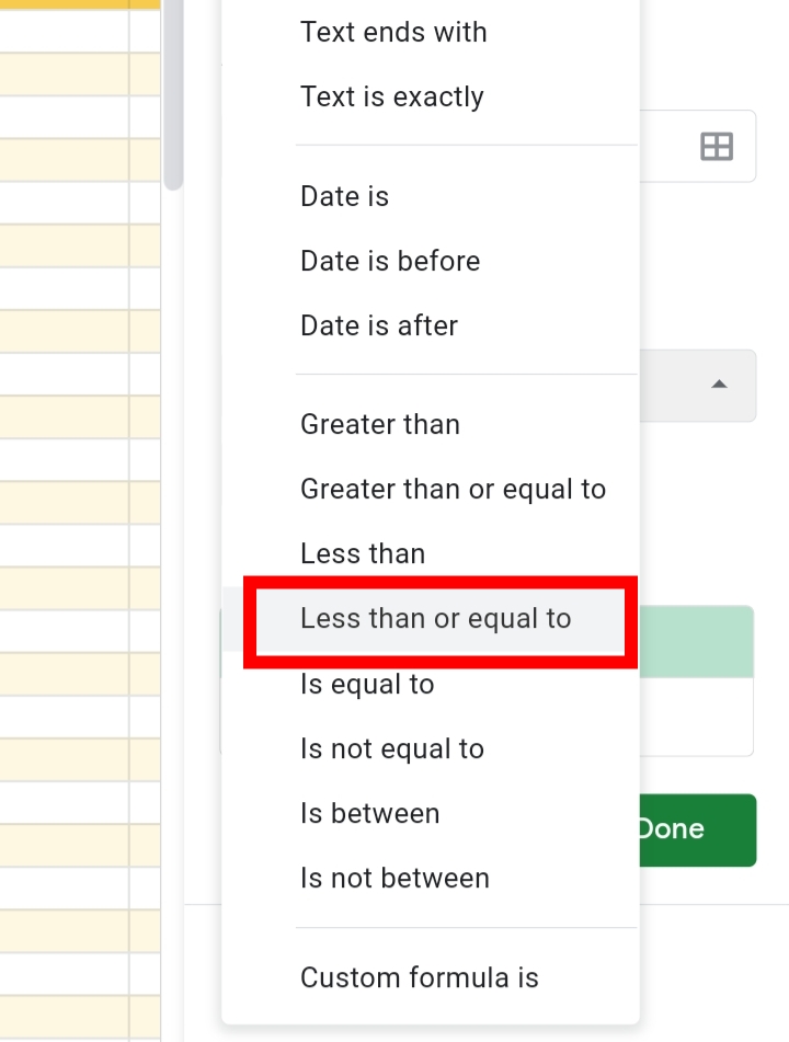
Step 7: In the text box, enter the formula
=SMALL($E$2:$E$50, 5).
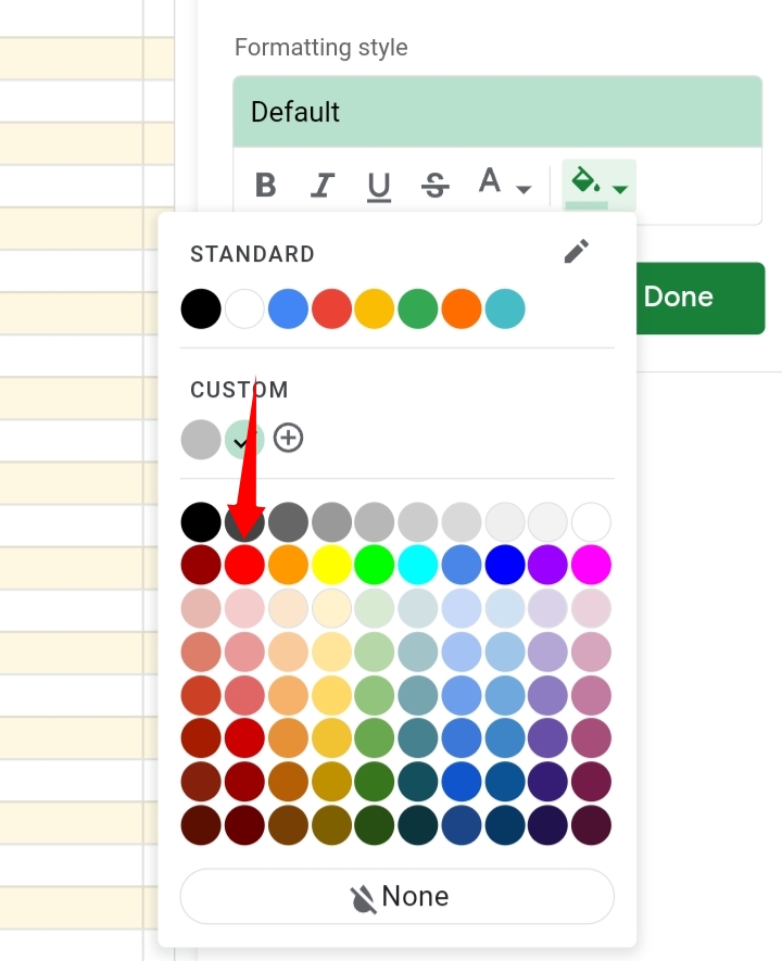
Step 8: You can customize how you want the highlight’s format to look. That’s if you don’t want to use the default format and colours. In this example, I selected Red.
Step 9: Click Done.
Now the highest and lowest values in that range are highlighted.
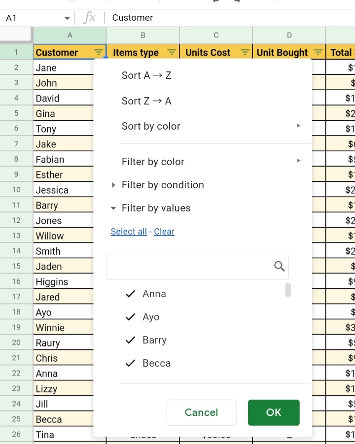
Create A Table In Google Sheets You Can Filter.
You can also add filters to your table for easy extraction of data.
Step 1: Highlight or select the data range of your table.
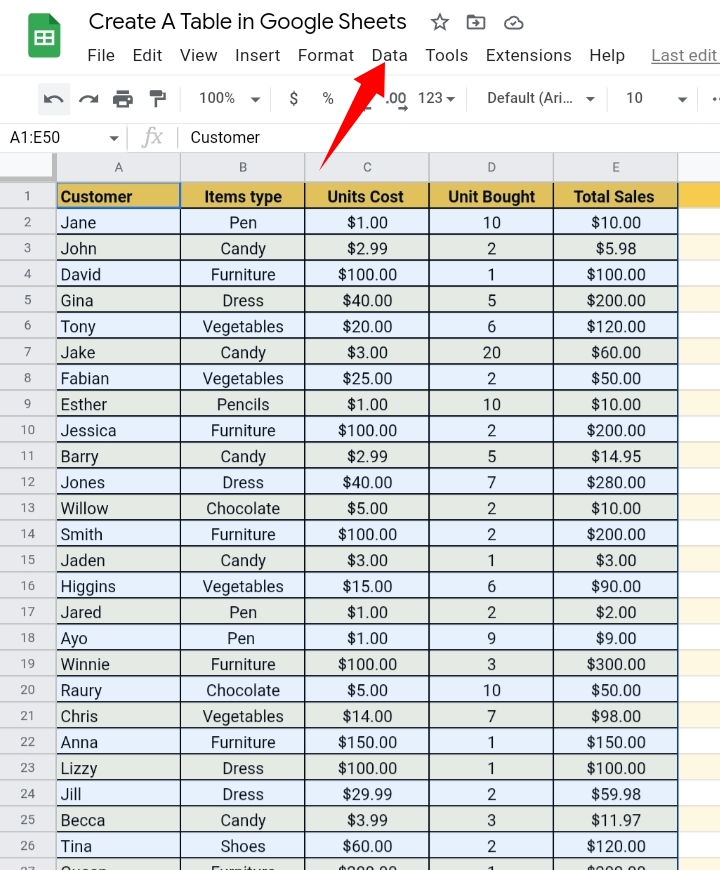
Step 2: Go to the toolbar and click on Data.
Step 3: From the drop-down list, select Create a Filter.
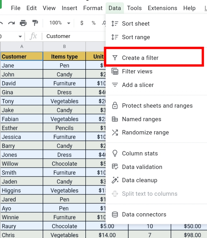
Step 3: From the list of available filters, select the filter of your choice.
Removing Formatting From A Table In Google Sheets.
If you don’t want your data presented in a table or you like the regular look in your worksheet you might as well remove all formats applied on your worksheet.
A straightforward way of doing this is by repeating the format process because it acts as a toggle switch but a preferred way is using the clear format option.
Step 1: Select the data range with the applied formats by clicking on the grey box at the top left corner of the worksheet.
Step 2: Go to the toolbar and select Format.

Step 3: From the drop-down list, select Clear Formatting. Alternatively, you can use a keyboard shortcut which is the Control key + \ (backslash).
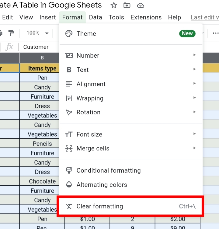
The above steps would successfully remove all formatting applied to your worksheet.
Frequently Asked Questions on How To Create A Table In Google Sheets (FAQs).
Here, we would treat some questions frequently asked by other Google Sheets users on how to create a table in Google Sheets.
Which button do I press to create a table in Google Sheets?
As mentioned earlier, there is no inbuilt feature or functionality to creating a table.
You’d have to follow the steps stated above to create a table on your worksheet.
How Do I Format A Table In Google Sheets?
There are multiple formats you can apply to format a table in Google Sheets and they are all thoroughly explained and treated in this guide.
But if you want a very easy way for this, you can use the borderline method which was discussed in the second section of this guide.
How Do I Make A Table Look Good In Google Sheets?
To add aesthetics and beauty to your table, you can include alternating colors in your header rows and cells.
For a more detailed description, please read the fourth and sixth sections of this guide.
Final Thoughts
These are the ways you can create and design a table in your worksheet. Since we have provided more than one way to do this, you can choose which one is more suitable for you.
Be adventurous and mix other formats into your table to give it a distinctive feel. If you have any other questions or suggestions, please let us know in the comment section.
Now you know in details about How To Make A Table In Google Sheets. I hope you found this guide helpful. Thanks for reading.


