When performing mathematical tasks and operations on your worksheet, you may come across a part of your dataset that you’ll need to divide.
Most times, we would like to divide two numbers without the result being formatted into decimal values.
Unlike other division functions, the MOD function is unique. The MOD function helps to prevent this by returning the remainder of the division if the division isn’t a perfect one.
In this tutorial, we are going to discuss and learn how to use MOD function in google sheets and in what case, can this function be applied.
What is MOD Function?
The MOD function is an inbuilt function in Google Sheets that returns the remainder value after two numbers are divided. It is also referred to as the Module Operator.
This function requires two arguments, which are the dividend and divisor. The MOD function takes the syntax below.
=MOD(dividend, divisor)
Where;
- The dividend is the number that is going to be divided.
- The divisor is the number that the dividend is divided by.
How Do You Use the MOD Function In Google Sheets?
The MOD function isn’t limited to just finding remainders, it is also used to find the last number in number string, prime numbers, odd and even numbers.
As stated earlier, the MOD function returns the remaining value after dividing the numbers.
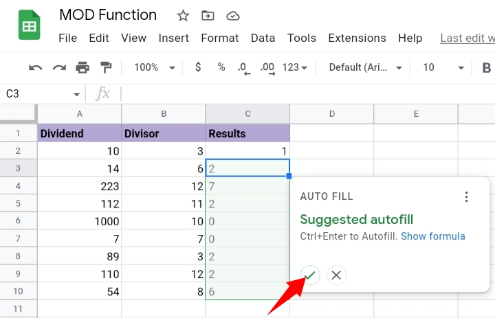
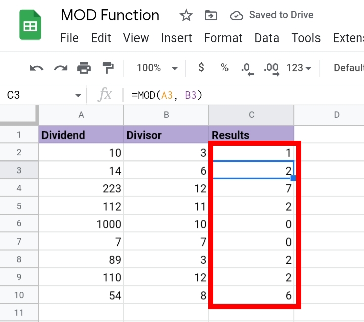
In columns A and B, we have a list of digits in each column from cells A2 to B10. In column C, we are going to divide the values into these two columns and return them to cells C2 to C10.
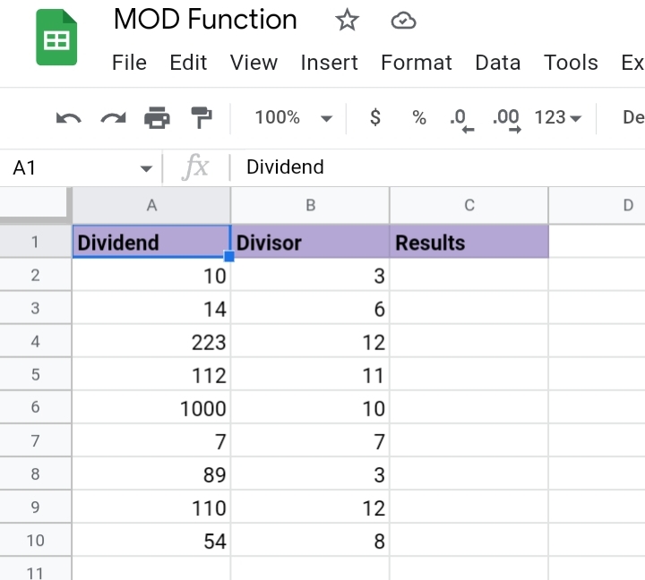
Here is how you use the MOD Function.
Step 1: In cell C2, you can either enter the values directly into the formula, like this =MOD(10, 3) or use their cell references like this =MOD(A2, B2).
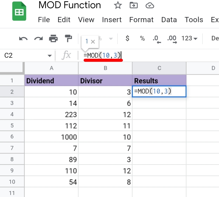
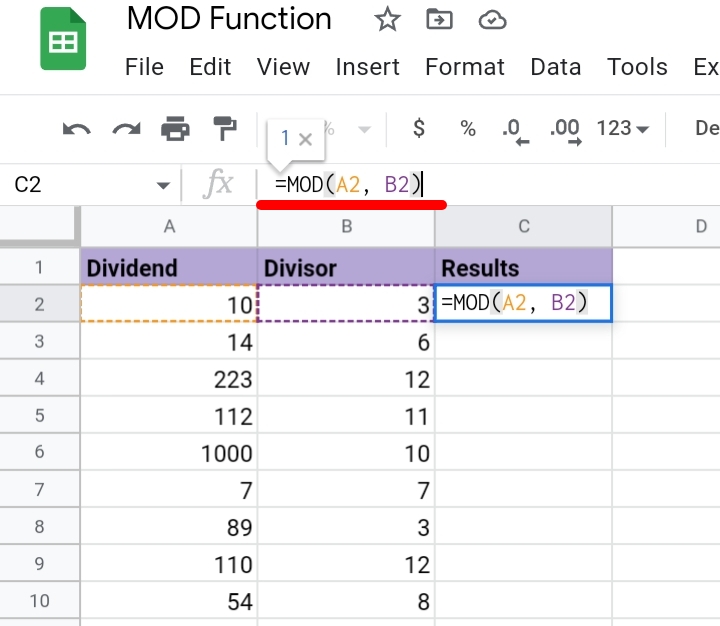
Step 2: Hit the Enter key on your keyboard and a value of one is returned to cell C2. Either way, the two methods return the same results.
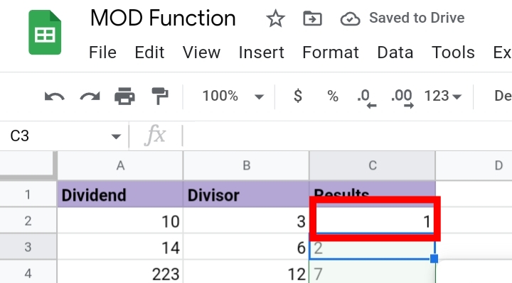
Step 3: To copy the formula into the other cells below, you can drag down the formula by using the fill tube on the bottom right of the cell or by accepting Google Sheets autofill suggestion.
Step 4: The remainder of these values are returned to column C.
What’s the Real-life Use of Google Sheets MOD Mathematical Function?
Here, we are going to understand how the MOD function can be used in a more dynamic approach in real-life situations.
The MOD function can form dynamic bonds with the ARRAYFORMULA and ROW functions. The formula takes the syntax below.
=ARRAYFORMULA(MOD(ROW(cell range), 2))
Other functions can combine with this formula to form something more dynamic.
For example, the FILTER and QUERY functions can be added to the syntax, in case you want to filter, query and extract specific values in the selected column.
When Should You Not Use The MOD Function in Google Sheets?
There are some instances where the MOD function won’t work on your worksheet.
- Dividing a digit by 0. Mathematically, dividing any number by zero would result in zero. This also applies to the MOD function.
- The MOD function also works only with integers. If the divisor or dividend is not an integer or whole number, the MOD function won’t work. In this scenario, the ROUNDDOWN function can be used.
What Are Some Similar Formulas to the MOD Function in Google Sheets?
- The percent operator, %, can also be used to find the remainder of two numbers.
- The ROUNDDOWN can be used. It is used to round down a number to the nearest figure.
- The ROUNDUP can be used. It is used to round up a number to the nearest figure.
Final Thoughts.
The MOD function is not common in Google Sheets, although it is very straightforward and may come in handy when working on a mathematical database.
If you’ve noticed the importance of this function and you agree with its usefulness, be sure to learn and practice it more frequently.
Also, experiment with other functions to come up with other dynamic combination formulas that may help you and other users in the Google Sheets Community.
Now you know How To Use MOD Function In Google Sheets. I hope you found this review helpful. Enjoy.


