When working on a dataset with multiple values and conditions, you may want to add up the values that apply to a particular condition on your worksheet.
To do this, you would use the SUMIF and SUMIFS functions. If you aren’t familiar with this function, it is quite easy to learn and understand.
Basically, the SUMIF function allows you to add up values that are based on a single condition. But when you need to add up values with multiple conditions, the SUMIFS function is used.
This article is a complete guide on how the SUMIFS function is used and the logic and explanation behind every application of the SUMIFS function. To get the most out of this guide, be sure to stick around to the end!
What Does the SUMIFS Google Sheets Function Do?
As said earlier, the SUMIFS function sums up values that apply to multiple conditions in your worksheet.
The function operates by analyzing the dataset within a specific cell range, then it extracts the values that satisfy the given condition, and then it adds these values together.
The final result is returned to the selected cell.
How to Use SUMIFS in Google Sheets
Before we start, we have to understand the syntax of this function and the parameters needed for its formula to work accurately.
The SUMIFS function takes the syntax stated below.
=SUMIFS(sum_range, criteria_range1, criteria1,[ criteria_range2, criteria2, … criteria_range_n, criteria_])
Where,
- The sum range is the cell range that contains the needed values.
- The criteria range1 is the cell range where you want to search for the first condition.
- Criteria1 is the first condition that criteria range1 searches for.
- The other included parameters (criteria_range2, criteria2) are not compulsory. They can be added when you have to search for other conditions.
- Criteria_range_n implies that you can add as many criteria ranges and their criteria as you want.
How To Use the SUMIFS Function in Google Sheets
The SUMIFS functions can be used in different ways. It can be used with texts, numbers, dates, wildcards, and operators as criteria.
Note that an array formula cannot be used with the SUMIFS function.
Now that we understand the dos and don’ts when using the SUMIFS function, we’ll practicalize it on a sample worksheet.
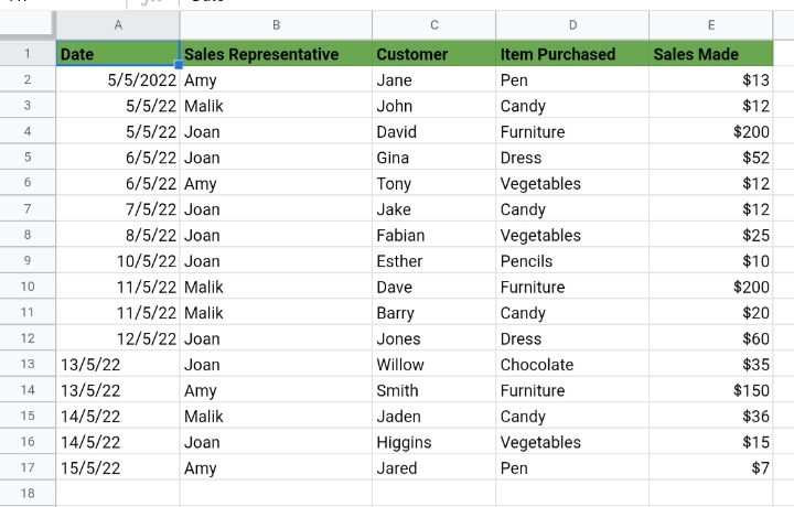
In the sample worksheet below, I have a dataset of purchase dates, sales representatives on duty, customer names, items purchased and the sales made in May.
I would show you to know the total of these transactions based on some conditions here.
I’ll show you some ways to use the SUMIFS function on your worksheet.
Using Text Conditions
In the first case, we want to know the total sales made on Dresses that were sold by Joan. That means we have two criteria. The Item Purchased is “Dress” while the Sales Representative is “Joan”.
Therefore, the required parameters would take the following values.
- Sum_range is the range of the sales made, that is, E2:E17.
- Criteria_range1 is the range of the sales representatives, that is, B2:B17.
- Criteria1 will be “Joan”.
- Criteria_range2 is the range of the items purchased, that is, D2:D17.
- Criteria2 is “Dress”.
The formula would look like this.
=SUMIFS(E2:E17, B2:B17, “Joan”, D2:D17, “Dress”)
1. Enter the above formula into an empty cell. This is where the result would be returned. In this case, I selected cell F3.
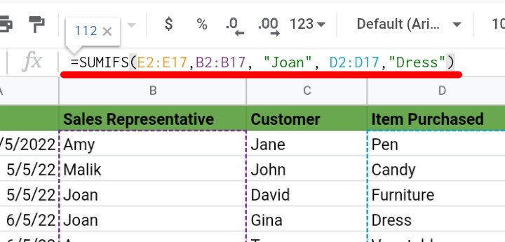
2. Hit the Enter key and the total sales made by Joan on dresses are returned into cell F3.
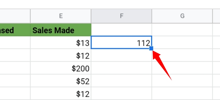
Explanation of the SUMIFS and Logic in This Formula
In case you don’t understand how the SUMIF formula returned that value, I’ll explain it properly here.
The SUMIFS function scanned the ranges B2:B17 and D2:D17, for cells that match the given criteria (Joan and Dress).
Then, when it finds a row that satisfies the conditions, the function moves to range E2:E17 to find the sales made on the item.
After that, it adds up the sales and returns the result in cell F3.
Using SUMIFS with Date Condition.
Another way to use the SUMIF function is to apply a date as its condition. Using the same worksheet, I want to use the dates as the criteria now.
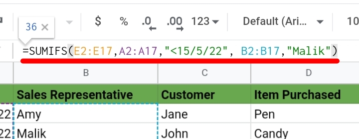
Let’s assume that I want to know the total sales made by Malik before May 15th 2022.
Now the conditions are: Date is “<15/05/2022” while the Sales Representative is “Malik”.
In this case, the parameters are
- Sum_range is the range of the sales made, that is, E2:E17.
- Criteria_range1 is the range of the date, that is, A2:A17.
- Criteria1 will be “<15/05/2022”.
- Criteria_range2 is the range of the sales representatives, that is, B2:B17.
- Criteria2 is “Malik”.
The formula would look like this.
=SUMIFS(E2:E17, A2:A17, “<15/05/2022”, B2:B17, “Malik”)
1. Enter the above formula into an empty cell. This is where the result would be returned. In this case, I selected cell F3.
2. Hit the Enter key and the total sales made by Malik before the 15th of May 2022, is returned to cell F3.
Explanation of the Formula.
The SUMIFS function scanned the ranges A2:A17 and B2:B17, for cells that match the given criteria (<15/05/2022 and Malik).
Then, when it finds a row that satisfies the conditions, the function moves to range E2:E17 to find the sales made before the specified date by Malik.
After that, it adds up the sales and returns the result in cell F3.
Using SUMIFS with Number Condition.
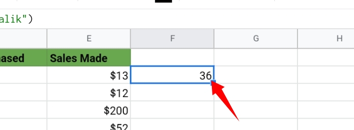
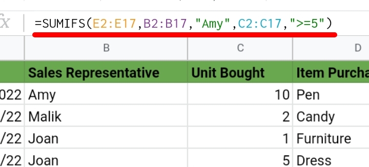
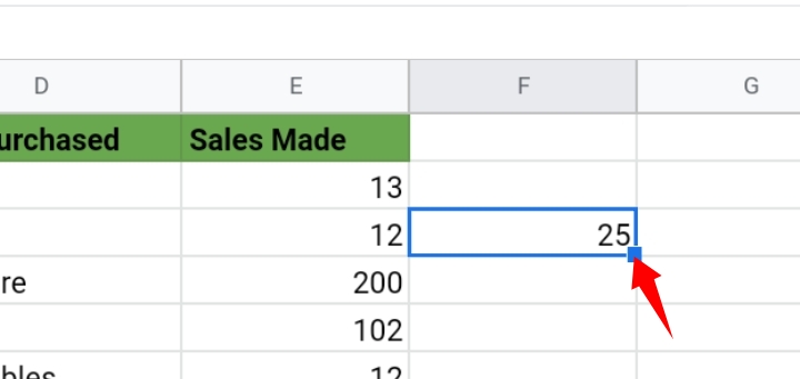
Lastly, you can use a number as a condition for the SUMIFS function. Let’s say we want to know the total sales made on some units sold by Amy that are more than or equal to 5 units.
That means we have two conditions, which are: units sold is “>=5”, and the Sales Representative is “Amy”.
In this case, the parameters are
- Sum_range is the range of the sales made, that is, E2:E17.
- Criteria_range1 is the range of the sales representative, that is, B2:B17.
- Criteria1 will be “Amy”.
- Criteria_range2 is the range of the units sold, that is, C2:C17.
- Criteria2 is “>=5”.
The formula used would look like this.
=SUMIFS(E2:E17, B2:B17, “Amy”, C2:C17, “>=5”)
1. Enter the above formula into an empty cell. This is where the result would be returned. In this case, I selected cell F3.
2. Hit the Enter key and the total sales made on units above 5 units by Amy, is returned into cell F3.
Explanation of the Formula
The SUMIFS function scanned the ranges B2:B17 and C2:C17, for cells that match the given criteria (Amy and >=5, respectively).
Then, when it finds a row that satisfies the conditions, the function moves to range E2:E17 to find the sales made on the units.
After that, it adds up the sales and returns the result in cell F3.
Multiple Conditions in One Column (SUMIFS OR Google Sheets Logic).
Google Sheets can’t use SUMIF to add multiple conditions that are in a single column. The easiest way to do this is by adding two SUMIFS calculations together. But each calculation should have different conditions but the same sum range.
Only then would you be able to sum multiple criteria in a single column in Google Sheets.
Frequently Asked Questions on Google Sheets SUMIFS (FAQs).
1. Can You Add Two SUMIFS Together? / Can You Use or With SUMIFS?
Yes, you can. It can be done by using a direct formula into two SUMIFS statements and adding them together. For example:
=SUMIFS(D2:D17, C2:C17, “True”, E2:E17″True”) + SUMIFS(D2:D17, C2:C17, “False”, E2:E17, “True”)
2. How Do You Do Sumifs With Multiple Criteria in Google Sheets?
Yes, you can. If there are multiple criteria in different columns, you can include these criteria in a SUMIF formula. Like in the calculations treated above.
=SUMIFS(E2:E17, B2:B17, “Joan”, D2:D17, “Dress”)
There are multiple criteria and ranges in one SUMIF formula.
Final Thoughts
The SUMIFS function is very dynamic due to its capability to accommodate multiple criteria and ranges in a single SUMIF statement.
This function would come in handy for technical sum calculations in Google Sheets. If you have any questions or suggestions, let us know in the comments section below and you’ll get a response soon.
Now you know about SUMIFS Function In Google Sheets. I hope you found this guide useful. Thanks for reading.


