As a frequent spreadsheet user, there are multiple functions created at your disposal to help you access and examine your data easily.
Amongst these functions is the FILTER function.
In this guide, I’ll explain the FILTER function properly. I will also show you how the FILTER function works and how it is used in Google Sheets.
What is the FILTER function in Google Sheets?
Before we dive right in, you should know what the FILTER function is. The FILTER function is a function that lets you filter or sort out values in your dataset that match your set condition(s) or criteria(rion).
Although there is built-in functionality that helps to filter data, Google Sheets has also provided a function for easier access and more dynamic results.
The syntax of the FILTER function is as stated below.
=FILTER(range, condition1, [condition2, …])
Where;
- The range is the cell range containing the data you want to filter.
- The condition1 argument is the first condition you want to filter in the selected range. It is mostly denoted as a column or row included in the entire range of the dataset.
- The condition2 argument is an optional parameter. You can add this argument to your formula in case you have an extra condition
Once these conditions are satisfied, the FILTER function returns a TRUE or FALSE statement. I’ll explain further in the next section of this guide.
FILTER Function Explained.
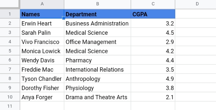
In the sample worksheet below, I have some names of some college students studying different courses at a university.
From columns A to C, I have their names, coursework and GPA listed respectively.
Here, I’ll show you how to use the FILTER function to extract some information on these students based on a single condition.
I’d like to see students with a GPA above 3.0. The formula would take the syntax below.
=FILTER(A2:C10, C2:C10> 3.0)
1. Enter the above formula into cell E2.
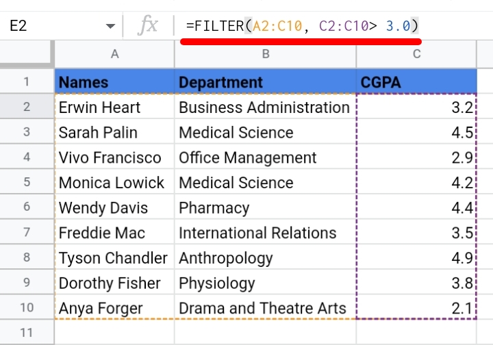
2. Press the Enter key on your keyboard and the filtered result is returned to the cell.
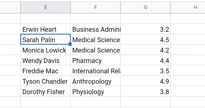
The FILTER formula scans the cell range A2:C10, for the students with a GPA that is greater than 3.0 in range C2:C1, then returns the names that match the stated criteria.
How To Use The FILTER Function in Google Sheets.
There are multiple ways to use the FILTER function in your worksheet. These methods differ with the number of conditions or the positions of the values in your dataset.
Method 1- Filter Records Based on Multiple Conditions.
The FILTER function can also accommodate more than one condition in its formula. It scans for values that match the two or more criteria given.
Using the previous worksheet, I want to check for the students in a particular department that has a GPA above 3.0.
The formula used takes the syntax below.
=FILTER(A2:C10, B2:B10=”Medical Science”, C2:C10 >3.0)
1. Enter the above formula into cell E2.
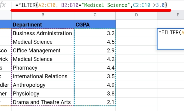
2. Hit the Enter key on your keyboard and the filtered result is returned to the cell.
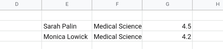
The FILTER formula scans the cell range A2:C10, for the students that are in the Medicine department in range B2:B10, with the GPA that is greater than 3.0 in range C2:C1, then returns the names that match the stated criteria.
These names return a TRUE statement which is why they are returned by the FILTER function.
Method 2 – How to Filter In Google Sheets for Top 3 or Top 5 Records
The FILTER function allows you to see the top 3 or top 5 values that match your condition in the dataset.
These numbers could be any number of positions from the top or the bottom of your cell range.
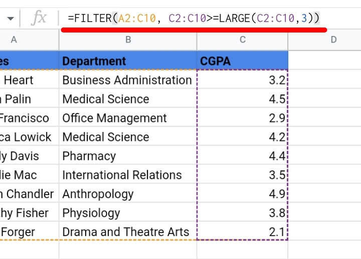
Supposedly I want to see the record of the top 3 students with a GPA of 4.0 and above.
The formula used takes the syntax below.
=FILTER(A2:C10, C2:C10>=LARGE(C2:C10,3))
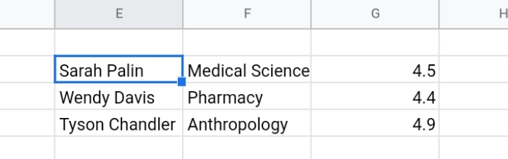
1. Input the above formula into cell E2.
2. Hit the Enter key on your keyboard and the filtered result is returned to the cell.
The formula is a combination of the FILTER and LARGE functions.
In this case, the LARGE function extracts the three highest values that meet the given condition.
You can also find the lowest values in the cell range by replacing the LARGE function in the formula with the SMALL function.
Method 3 – How to Use Filter Function In Google Sheets to SORT the Filtered Data.
The SORT function can also collaborate with the FILTER function to sort and arrange the returned data.
You can choose to either arrange your data in ascending or descending order.
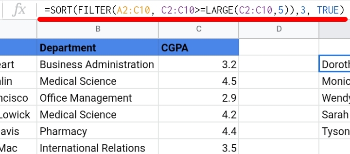
For instance, I want to filter the top 5 students with the highest GPA in ascending order.
The formula is arranged like this.
=SORT(FILTER(A2:C10, C2:C10>=LARGE(C2:C10,5)),3, TRUE).
1. Enter the above formula into cell E2.
2. Hit the Enter key and the filtered result is returned to the cell.
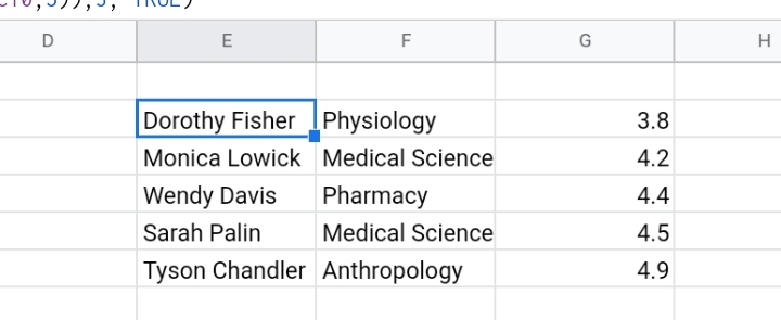
So here is how the formula works. The FILTER function returns the values that have the conditions met as a TRUE statement.
Then, the SORT function takes the returned statements and arranges them based on column C.
The TRUE parameter in the above formula helps to indicate the order of the sorted data.
If you want the order of your data arranged in descending order, you would replace the TRUE argument with FALSE.
NOTE: A Not Available (#N/A) error would be returned if the FILTER function does not see any value that meets the required conditions.
Method 4 – Filter All Even Number Records.
The FILTER function is very dynamic. You can also use it to filter the number of rows. Not all rows in your worksheet are used in your data.
You may want to remove some blank rows in between your data.
This is done by using the FILTER function to place the odd or even number rows in one place.
For instance, you have a worksheet with some blank rows in the even-numbered rows and you may want to filter these rows in the dataset.
To do this, you’d use the formula below.
=FILTER(A2:A10, MOD(ROW(A2:A10)-1,2)=0)
If you want to filter the odd-numbered rows out, this formula is used.
=FILTER(A2:A10, MOD(ROW(A2:A10)-1,2)=1)
Frequently Asked Questions on the FILTER Function in Google Sheets.
1. Can I test multiple conditions inside a Google Sheets FILTER function?
Yes, you can. For a more detailed explanation, you can read the fifth section of this guide!
2. Can I test multiple columns in a filter function?
Yes, you can. To do this, you need to add the columns as additional conditions to the formula.
For instance, the formula below has two different column ranges (A2:A5 and B2:B5) in a single formula.
=FILTER(A1:B5, A2:A5 > 50, B2:B5 > 50)
This formula would return the values that fall under these column ranges if they meet the required condition.
3. Can I reference a criteria cell with the Filter function in Google Sheets?
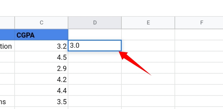
Yes. All you need to do is to use a cell reference as the condition of the FILTER function. That is, you have to enter the condition into an empty cell.
To prevent an #N/A error, ensure that there are no special characters or extra spaces after the entered condition.
For instance, I have some names of some college students studying different courses at a university. From columns A to C, I have their names, coursework and GPA listed respectively.
I’d like to see students with a GPA above 3.0.
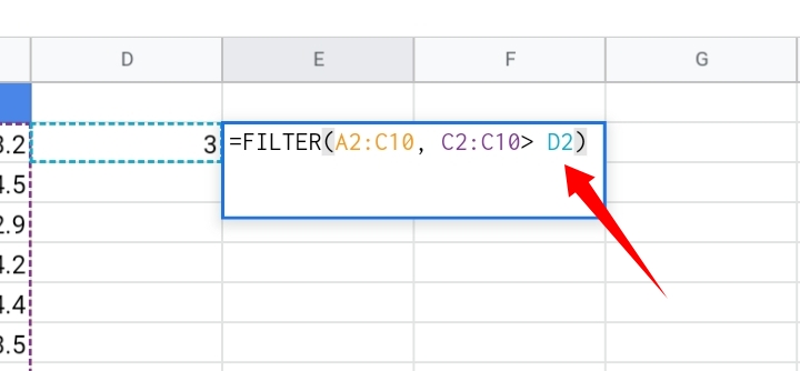
Instead of entering the condition directly into the formula’s syntax like this =FILTER(A2:C10, C2:C10> 3.0), I can enter the condition (3.0) into an empty cell, like cell D2 and make it serve as a cell reference.
Therefore, the formula would be =FILTER(A2:C10, C2:C10> D2)
4. Can I Do a Filter of a Filter?
Yes, you can. But using the FILTER function twice in a single formula can be confusing and may result in a lot of errors if you are not familiar with the method.
There is a great way to do this effectively with no hassle. That’s the use of the VLOOKUP function.
Final Thoughts
The FILTER function is the goto function whenever you have to filter or extract valuable information from your worksheet.
It is also dynamic so whenever you make an adjustment or change to the dataset, it automatically recalculates and accommodates the change instantly.
You can also get adventurous and combine the FILTER function with all other functions in your worksheet. This would increase your work output and efficiency.
I hope you found this guide beneficial. Thanks for reading.


