Although the strikethrough format is mostly utilized in document apps like Google Docs and Microsoft Word, it can be used in Google sheets to cross out or cancel out data without it being completely removed from the cell.
In this tutorial, we are going to learn what the strikethrough format is and how to add Strikethrough Format in Google Sheets and also how we remove this Strikethrough Format in Google Sheets.
What is a Strikethrough?
A strikethrough is denoted by a straight line cutting across a word or group of words in a selected cell, signifying removal or mistakes but not completely removing the word from the cell as the word can still be seen by the user.
This tool is frequently used to cancel out or cross out words from a list of words. The list of words could be a to-do list, a catalog, a timetable, an agenda or an order of the day.
The strikethrough majorly shows that the crossed-out word or agenda has been implemented successfully by the user.
Four ways are used to add strikethroughs to your Google sheet.
Method 1: Adding Strikethrough with the Format Drop-Down menu.
As a Google Sheet user, you are pretty much familiar with the functions of the Format tool on the toolbar.
Well if you aren’t, the format tool contains features that are used to improve visibility, text style and design of data in a worksheet.
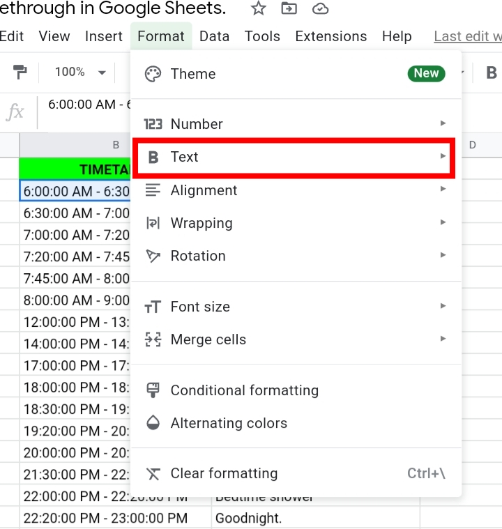
These features include Theme, Number, Text, Alignment, Text Rotation, Wrapping, and Conditional formatting. Under the Text tool, are the bold, italic, underline, and strikethrough formats.
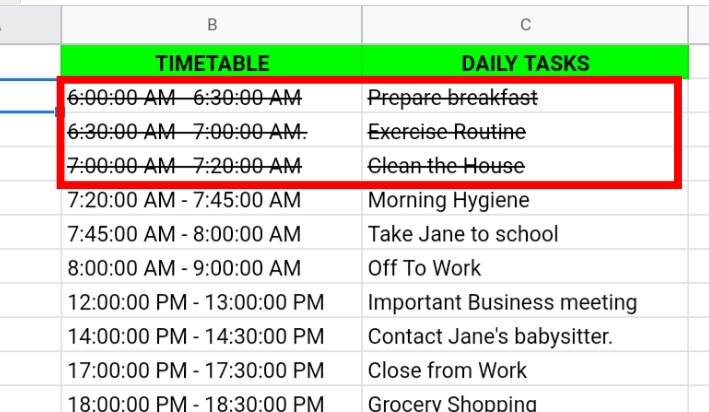
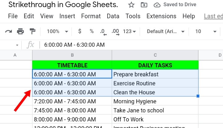
In the sample worksheet below, we have a list of daily chores and activities that we need to fulfill.
Some tasks are completed already while some aren’t, so we employ the strikethrough format to strike out completed tasks.
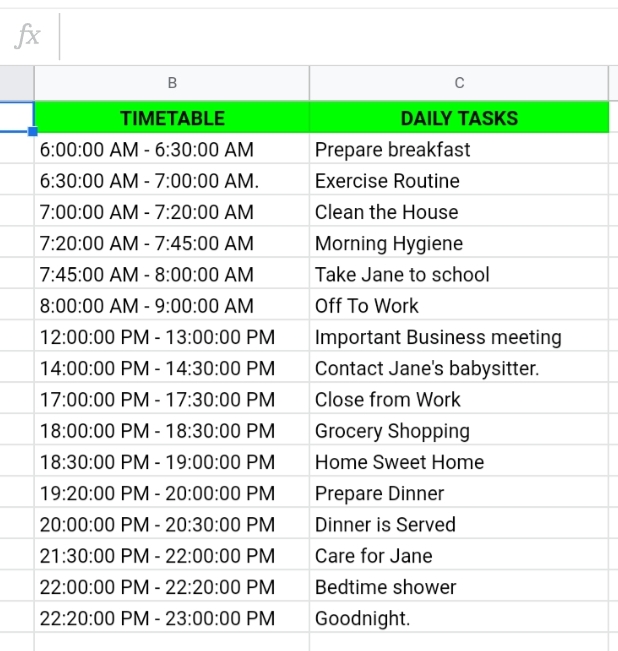
By following the steps below, you can apply a strikethrough to a text on your worksheet.
Step 1: Select or highlight the cell or range of cells on your worksheet.
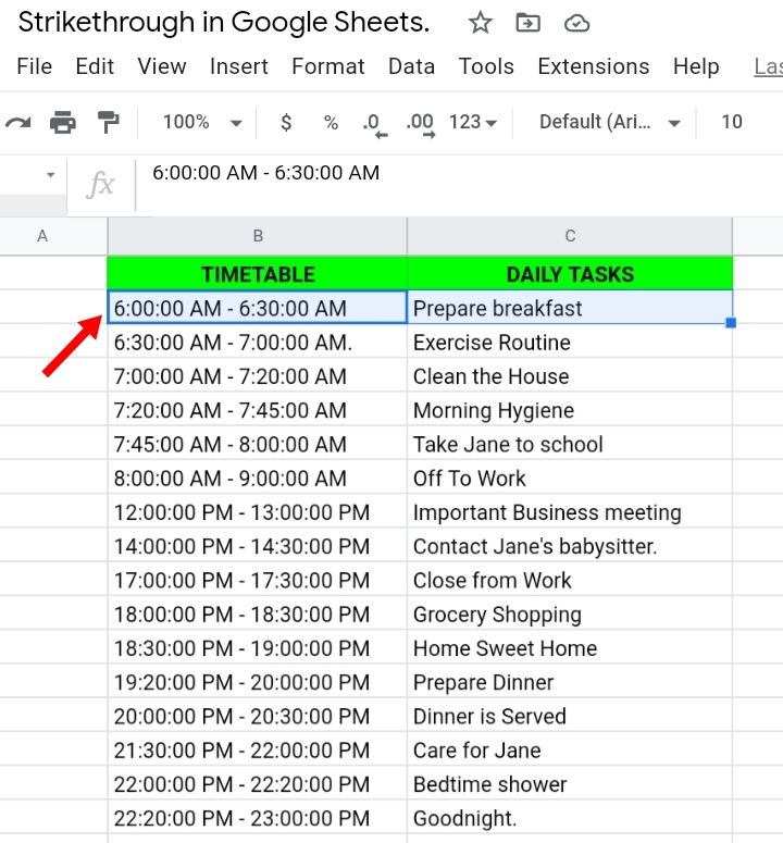
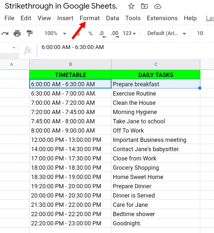
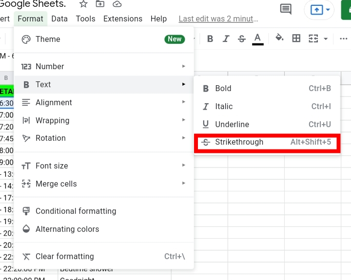
Step 2: On the toolbar, click on Format.
Step 3: A drop-down menu is produced under format, displaying the major features it entails. Click on Text.
Step 4: Under Text, are four other tools which are Bold, Underline, Italics, and strikethrough. Select strikethrough.
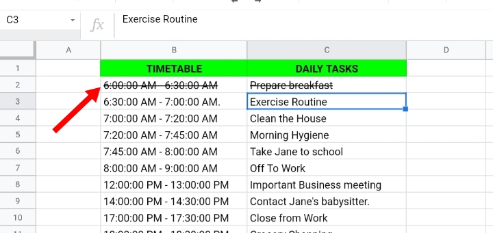
Step 5: The selected cell has its texts crossed out on the worksheet.
Method 2: Keyboard Shortcut to Apply Strikethrough in Google Sheets.
If you like easy, efficient and quick shortcuts then this method is just for you. Unfortunately, users with mobile devices with capacitive or sensitive displays can’t implement this method due to the absence of a keyboard. Users with desktop computers and laptops would enjoy this method more.
- Windows – Shift key + Alt key + 5. Press and hold the shift and alt keys, then click number five.
- MacBook – Command key ⌘ + Shift key + X.
With these shortcuts, strikethroughs are added to the selected cells.
Method 3: Add Strikethroughs through the Toolbar.
For those who cannot use the keyboard shortcuts, this is also a shortcut that is compatible with touch screen devices and is done in a few clicks.
Step 1: Select the cell or cells you want to work with.
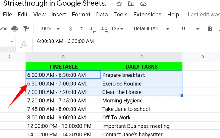
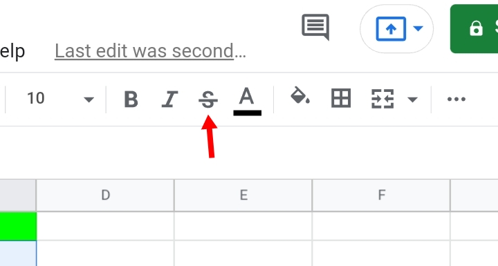
Step 2: Go to the top right of the worksheet. Little icons denoting different tools are presented there. Select the strikethrough icon as seen below.
Step 3: The selected cells have their texts crossed out of the cell.
Method 4: Add Strikethrough with Conditional Formatting.
In a case where you have a large schedule or timetable and you want to strike out data based on given criteria, conditional formatting is used.
Conditional formatting also works in collaboration with checkboxes in Google Sheets. Therefore, in the sample worksheet below, we would create checkboxes with the insert tool, and then we would add strikethroughs with the conditional formatting.
Step 1: Select a cell or highlight a range of cells.
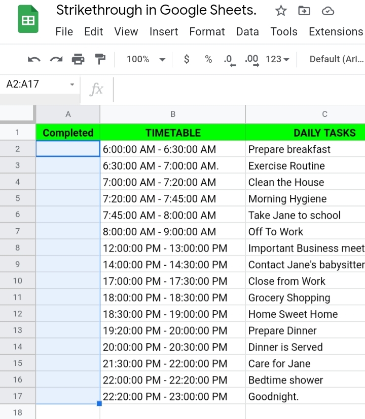
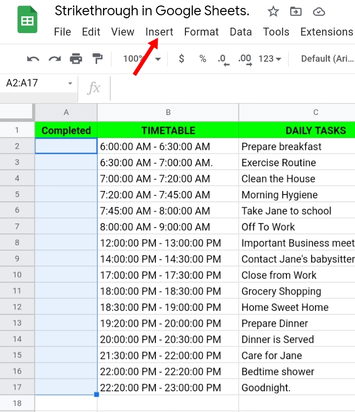
Step 2: Select Insert on the toolbar.
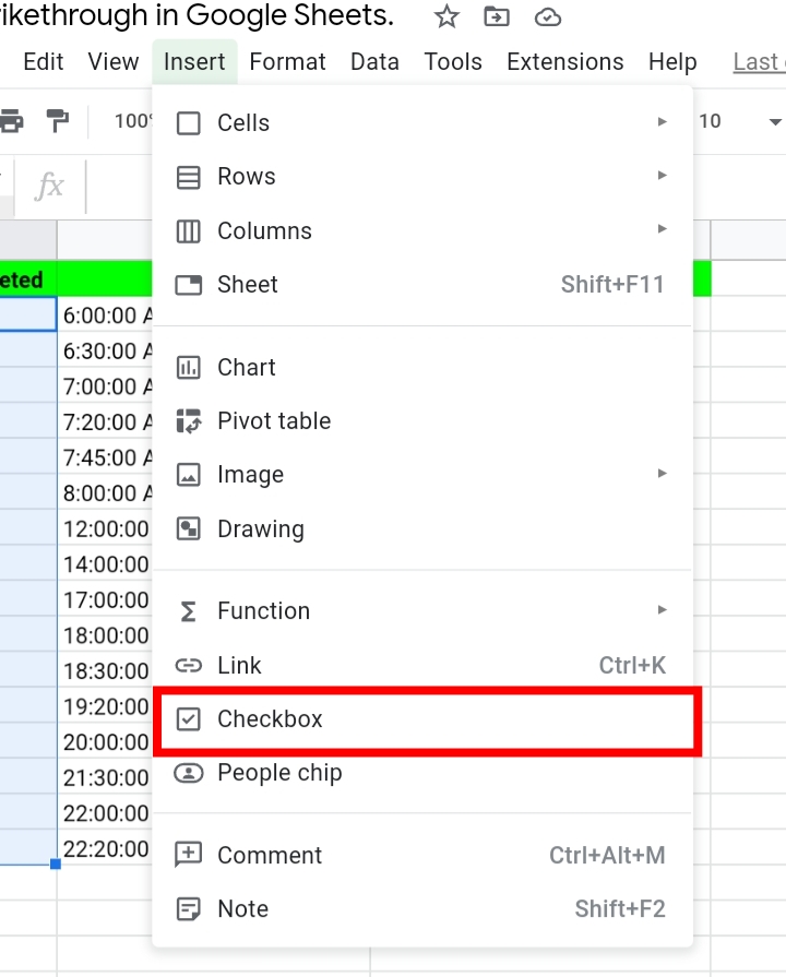
Step 3: A drop-down menu is produced, displaying a list of options. Click on the Checkbox option.
Step 4: Checkboxes are inserted in the selected cell or cells.
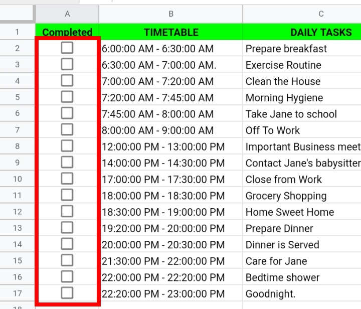
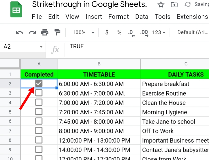
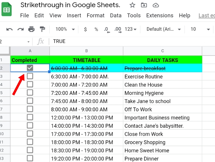
If you click on the boxes, a tick sign appears in the checkbox but it doesn’t cancel out the text in the cell. This is where Conditional Formatting comes in.
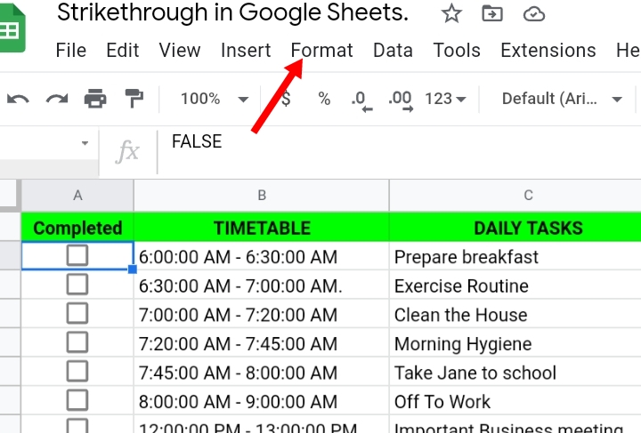
Step 1: Click on Format on the toolbar.
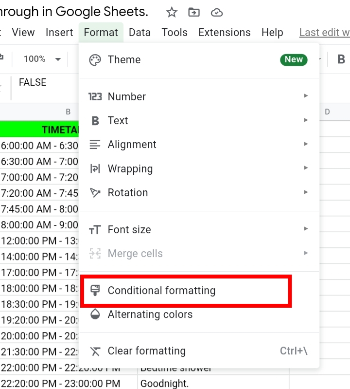
Step 2: Select Conditional formatting from the drop-down menu.
Step 3: The Conditional formatting tab is generated on the right side of the worksheet.
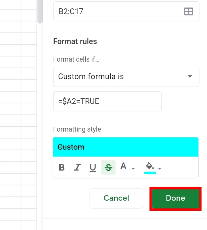
Step 4: Select Apply to Range. Select the data range of cells which is B2:C17.
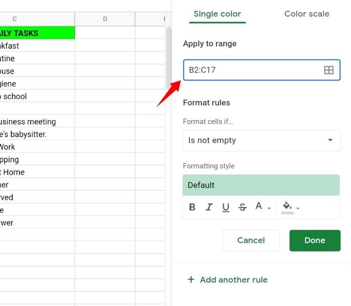
Step 5: Now, we are going to create rules and conditions for the format. Click on Format cells if.
Step 6: A drop-down menu is displayed. Select Custom Formula Is from the menu.
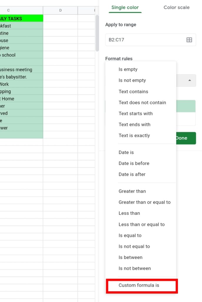
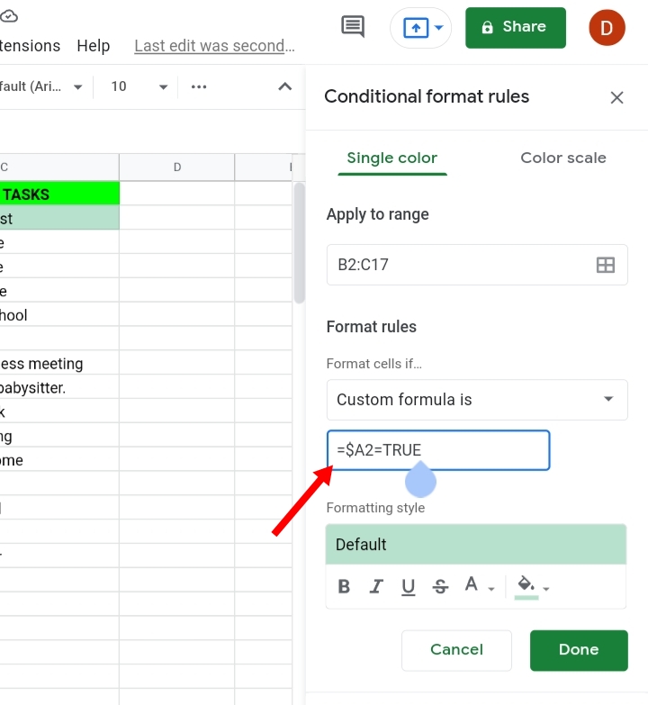
Step 7: In this section, we are going to create a formula that tells the format when to add a strikethrough to the worksheet. So if a checkbox is true and an unchecked box is false, then using a checkbox in cell A2 as a cell reference, the formula takes the syntax below.
=$A2=TRUE
The dollar sign in the formula locks the cell reference so it could be applied to all the cells in the range. This means that if a box is checked, a strikethrough should be added to the cell.
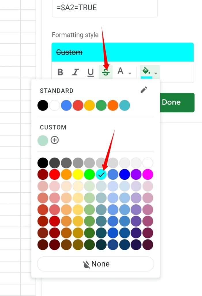
Step 8: This is the main aspect here, where we customize and change the formatting style.
Step 9: Click on the strikethrough icon here. You can also change the text and fill colors.
Step 10: Click Done.
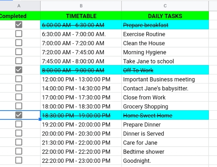
If you click the box, the task is crossed out and highlighted in the selected fill color.
Removing Strikethrough in Google Sheets.
We’ve discussed how to add strikethroughs to your worksheet, but what if you want to remove them? Don’t fret about it. The same methods used above to add strikethroughs are also used to remove them. If you want to remove strikethroughs from a worksheet,
- Select the cell or range of cells.
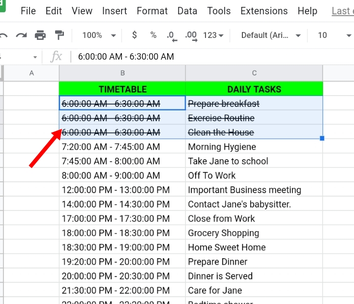
- Use any of the methods stated above like the shortcuts, format menu or strikethrough icon directly on the toolbar.

If the strikethrough was added by conditional formatting, you’d select the formatted cells or range of cells.
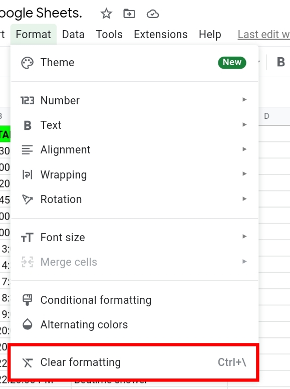
- Click Format on the toolbar.

- Click clear formatting here. All strikethroughs inserted are removed.
Final Thoughts.
Strikethroughs are necessary mechanisms that aid clarity and orderliness in task worksheets. Although it’s mostly used in word documents, it’s also quite efficient in spreadsheet documents too. I hope you found this tutorial informative. Thanks for reading.


