You may have observed that decimal figures with several numbers after the decimal point are frequently rounded off in Google Sheets.
In most circumstances, this is preferable because it ensures that the value does not cross the column border into the subsequent cell, making your spreadsheet look messy.
However, if you’re working with scientific data, where precision to the least substantial number is crucial, this could be a problem. Your number may be shown in exponent format in some instances.
How to Disable Rounding in Google Sheets – 2 Easy Methods
- TRUNC Function
- Cell Formatting
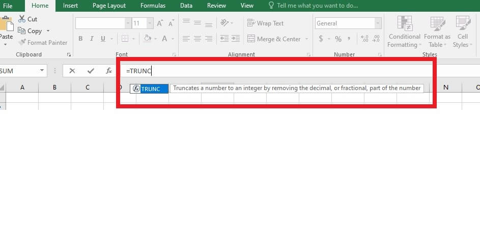
TRUNC Function
Truncate (TRUNC) is a Google Sheets function that displays decimals without rounding down or up. Any decimal points that aren’t visible keep their value; they’re just hidden.
This is the most straightforward way to display precise figures without having to establish a specific number form.
It’s also quite easy to use. Simply copy and paste the script into the place where you would like the unrounded number to appear. The following is the code’s syntax:
Code Format:
‘=TRUNC(Value,[Places])’
- The command line ‘=’ indicates that this would be a format script to Google Sheets.
- The function ‘TRUNC’ specifies whether or not whatever is provided will be truncated.
- ‘Value’ refers to the amount you want to display that would not be rounded.
- The amount of decimal points you want to see is indicated by ‘Places.’
Furthermore, You can put variables in the value area to avoid manually entering numbers.
For example, the formula =TRUNC would be used for the truncation of the numerical value in cell A1 to five decimals (A1,5). If you want to see the truncated result of the result of two cells, type =TRUNC(A1+A2,5) into the formula.
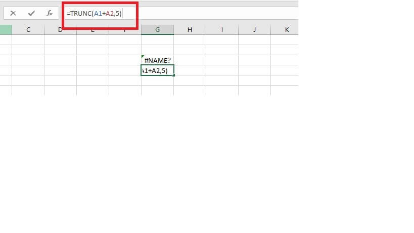
Another script can alternatively be used as the value. The total of numerous cells, such as A1 through A10, will be expressed as =SUM (A1:A10). =TRUNC(SUM(A1:A10),6) would be the formula to display it shortened to six decimal places. For the following step, simply leave off the equals sign to avoid an error.
When entering the equation, be cautious of the syntax you employ. Although the logic is not case sensitive, the function will produce an error if a comma or parenthesis is misplaced.
When you get a #NAME issue, it means Google Sheets is having problems finding a value you provided. By selecting it and glancing at the number window directly above the pages, you can double-check your code.
This is the long message box to the middle of which is fx. If a cell has an equation, it will be shown here at all times.
A Quick Recap:
- You can stop your values from rounding with the TRUNC function.
- Type the syntax ‘=TRUNC(Value[Places])’
- Put the cell value in the ‘Value’ and insert the limit for decimals in ‘Places’.
- This way you can stop your values from rounding.
Check out How To Change Row Height In Google Sheets.
Cell Formatting
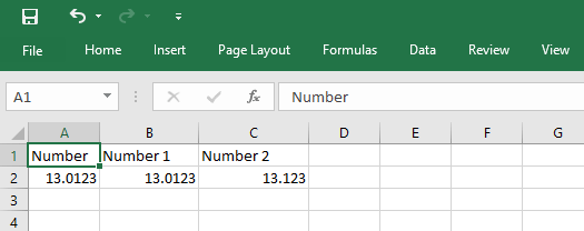
This approach has a direct impact on the cell, formatting it to show additional decimals. It’s as easy as picking the cell/cells you would like to format and pressing the ‘Increase decimal places’ option. This button is located in the toolbar as follows:
Every time you push this key, the underlying number will be displayed to one additional decimal point in the specified cell.
As seen in the instance below, hitting the key once will show the complete number recorded in cell A3, whereas pressing the button again will display the actual number recorded in cell A4.
In this manner, you can see your complete number without having to round it.
Why Is Google Sheets Rounding Up?
There could be various causes for your Google Sheets numbers being rounded. The following are a few possibilities:
- Number More Than 11 Digits.
- Cells Might be Formatted to Display Lesser Number of Digits.
Number More Than 11 Digits
By definition, Google Sheets allows just 11 digits (total) to be shown in a cell. Any additional digits are trimmed off.
To put it another way, the fundamental number remains entire and unaffected. When you’re using the cell value in a calculation, the complete original number (including the digits following the 11th) is used, not simply the numbers in the cell.
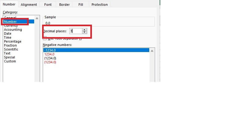
Cells Might be Formatted to Display Lesser Number of Digits.
Aside from that, certain cells’ default formatting may round off a numeric integer to only one or two decimal places.
Your numbers will most likely round off to two (or sometimes more) digits if your cell is structured in one of the following categories:
- Accounting Format
- Financial Format
- Number Format
- Currency Format
When one of the aforementioned formats is selected, values are automatically rounded to 2 decimal values. Even if they are set to show more than 2 decimal places, the decimals will be rounded out in the end.
Your decimals will be rounded off to a whole number if your cell is structured in the Currency (rounded) style.
Final Thoughts
Hope for now you can easily Stop Your Google Sheets From Rounding. Thanks for reading this article. Best of luck.


