In Google Sheets, you can remove any letter based on its position in the text string. This is most important for creating abbreviations and finding common characters in the group of words. This is done with the LEFT, RIGHT and MID functions.
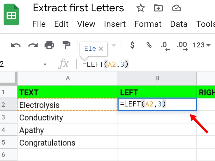
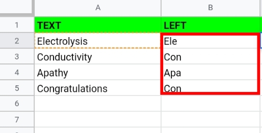
To extract the first few letters from the left, use the formula =LEFT(string,(number of characters).
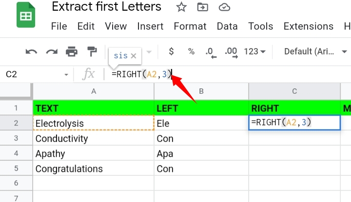
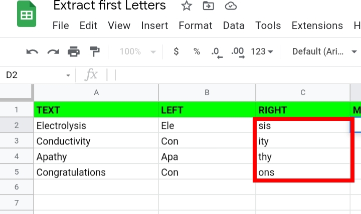
To extract the last few letters from the right, use the formula =RIGHT(string, (number of characters).
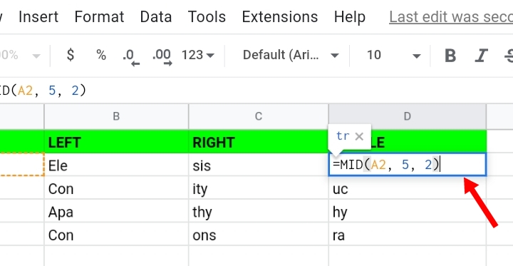
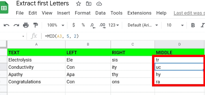
To extract the middle characters in the string, use the formula =MID(string, starting at, extract_length).
Starting at means the number where you want the counting to start.
Extract length means the number of letters you want to extract.
Normally, using the SPLIT, LEFT and JOIN functions and copying the formula into the remaining cells, we can extract the first letters in Google sheets.
The formula takes the syntax below.
=JOIN( ” ‘, ARRAY FORMULA(LEFT(SPLIT(cell reference, ” “), 1))).
Explanation.
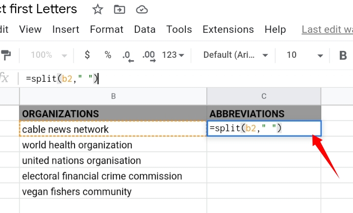
The SPLIT function intersects the text into three parts. =SPLIT(cell reference, ” “)

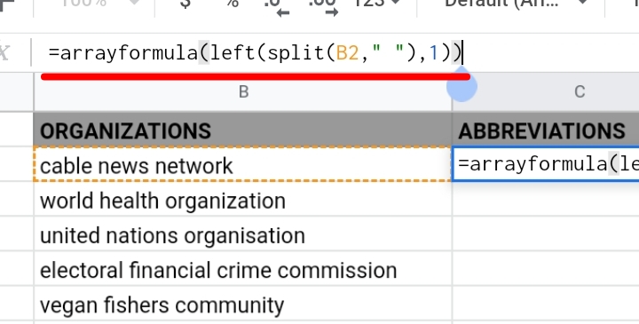
The LEFT and ARRAY FORMULA functions pull out the first letter in the text from the left side of the cell.
=ARRAYFORMULA( LEFT( SPLIT( cell reference, ” “), 1))

Finally, the JOIN function joins the extracted left characters to form a single string.
=JOIN( ” ‘, ARRAY FORMULA(LEFT(SPLIT(cell reference, ” “), 1))).
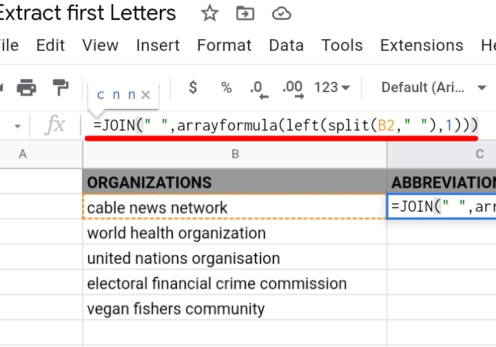
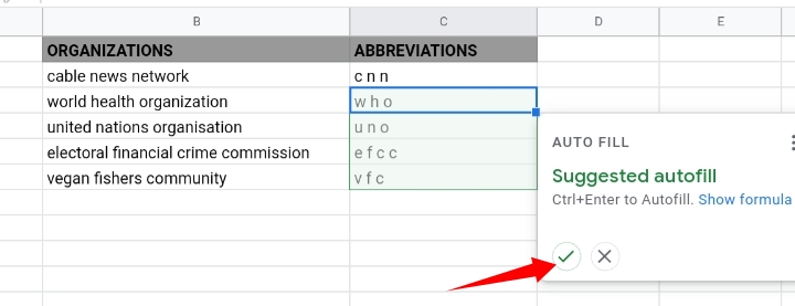
Click on the suggested autofill to copy the other texts into their respective cells.
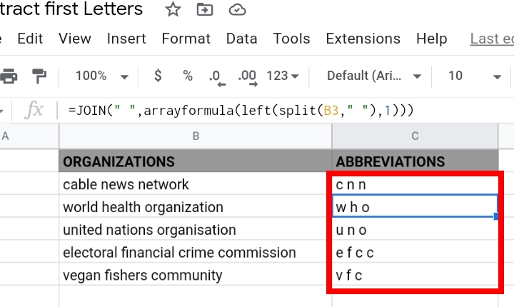
This method is the non-array technique. It Is considered the best way for pulling out characters but this method is regarded as a difficult one due to its inability to code an array formula.
In this tutorial, we are going to discuss the two array formulas to extract the first character of each word in Google sheets.
Two Array Formulas to Extract the First letter of Each word in Google Sheets.
There are two array formulas, one is easy while the other is somewhat complicated but we are going to explain the formulas best to your understanding.
Formula One.
This is the first method. It is highly recommended to those who aren’t concerned about the change of letter case because this formula converts the first letters of each word in the string, to capital letters.
In the sample worksheet below, there are names of global organizations in lower case.
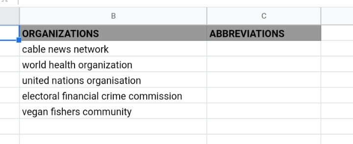
We want to extract their first letters to form abbreviations in upper case letters.
Step 1: The text in cell B2 is in lower case. With the PROPER function, the first letters would be in upper case and the others are lower case characters.
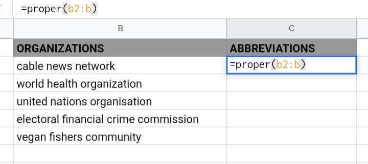
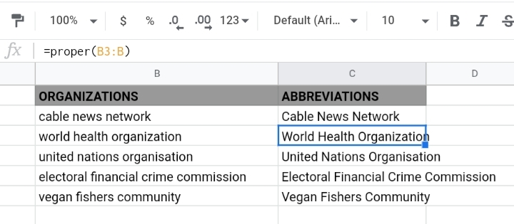
Step 2: The REGEXREPLACE function would extract the first characters in the text. The array formula takes the syntax below.
=ARRAYFORMULA(REGEXREPLACE(PROPER(B2), ” [^A-Z]+”, ” “))
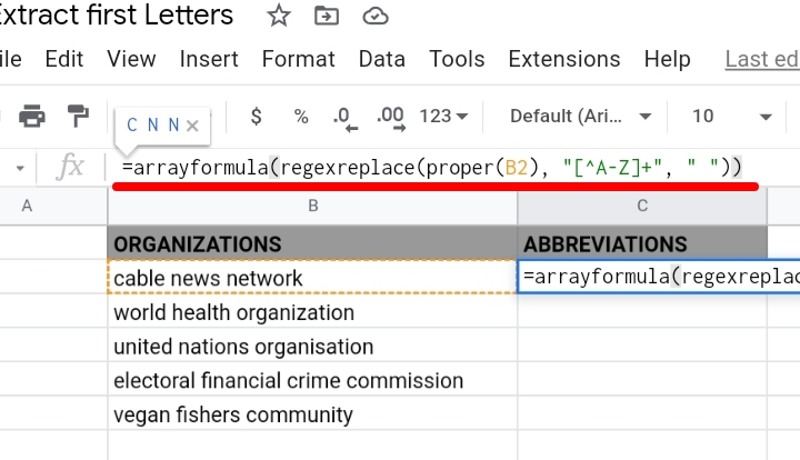
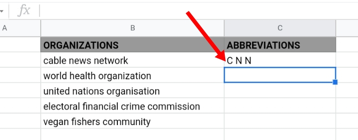
Step 3: Input the formula into cell C2. Click Enter and the extracted letters are changed to capital letters.
Formula Two
This is the complex formula. The texts in the cell undergo a series of steps with the FILTER, SPLIT and LEFT functions before the QUERY and TRANSPOSE array formulas extract the first letters.
This formula won’t change the letter case of the extracted characters.
Step 1: Use the FILTER function to skip blank cells in the worksheet.
=FILTER (B2:B, B2:B <>” “)
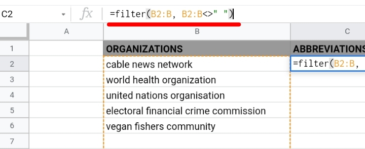
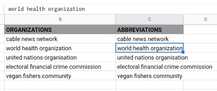
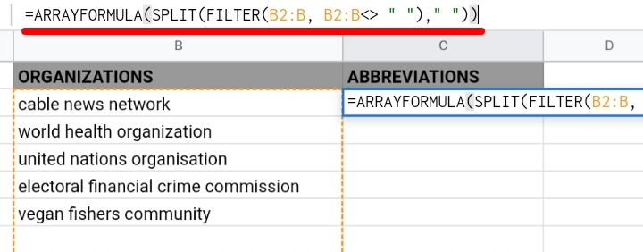
Step 2: Use the SPLIT function to separate the words in the string into cells.
=ARRAYFORMULA(SPLIT(FILTER(B2:B, B2:B <> ” “), ” “))

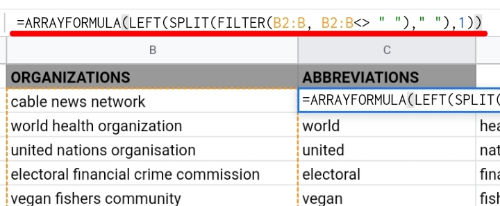
Step 3: Use the LEFT function to extract the first character from the left side of the text string.
=ARRAYFORMULA(LEFT(SPLIT(FILTER(B2:B, B2:B <> ” “), ” “), 1))

Step 4: Use the QUERY function to consider all cells in the range of titles and join them together into a single cell. The QUERY function works in conjunction with the TRANSPOSE function to change the exposure and combine the characters.
=TRANSPOSE( QUERY( TRANSPOSE( ARRAYFORMULA( LEFT( SPLIT( FILTER( B2:B, B2:B <> ” “), ” “), 1))), , 9^9))
Input the formula into cell C2 and press Enter.

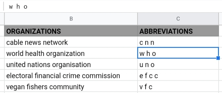
The letters have spaces in between them. To remove them, we use the SUBSTITUTE function.
=ARRAYFORMULA( SUBSTITUTE ( TRANSPOSE( QUERY ( TRANSPOSE( LEFT( SPLIT( FILTER( B2:B, B2:B<>” “), ” “), 1)),, 9^9)), ” “, ” “))
The spaces are removed from the letters. They are still placed in lower case, if you want to change them to upper case, use the Upper function.
With the formulas above, the first letters in the text are extracted.
Final Thoughts.
Now you know how to Extract the First Letter of Each Word in Google Sheets.
That’s all for this topic. If you have any other formulas that are used to extract letters, do let us know in the comment section. Thanks for reading.


