The Conditional formatting tool is an inbuilt feature in Google Sheets that selects and highlights important aspects of your worksheet based on a set condition or formula.
When you have conditional formatting applied on a specific range or column and you want it applied to another column or another sheet entirely in your workbook, you need to copy the format originally applied.
In this tutorial, we are going to discuss the methods used to copy the conditional formatting into other columns and sheets in your document In Google sheets.
Method 1: Using Paste Special
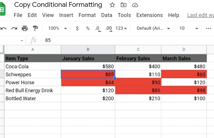
This is the first method used to copy conditional formatting into other cells. In the worksheet below, we have a list of items and the total amount sold on each item from January to March 2022. A set condition has been placed on column B, which represents the sales made in January.
Every sale of less than a hundred dollars is formatted and highlighted. So we want to copy this format into the other columns in the worksheet by using the Paste Special method.
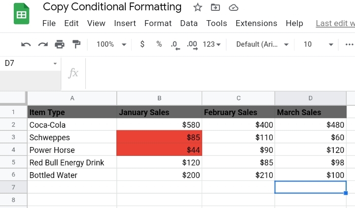
Step 1: Select all formatted cells in column B which have the conditional format applied to it.
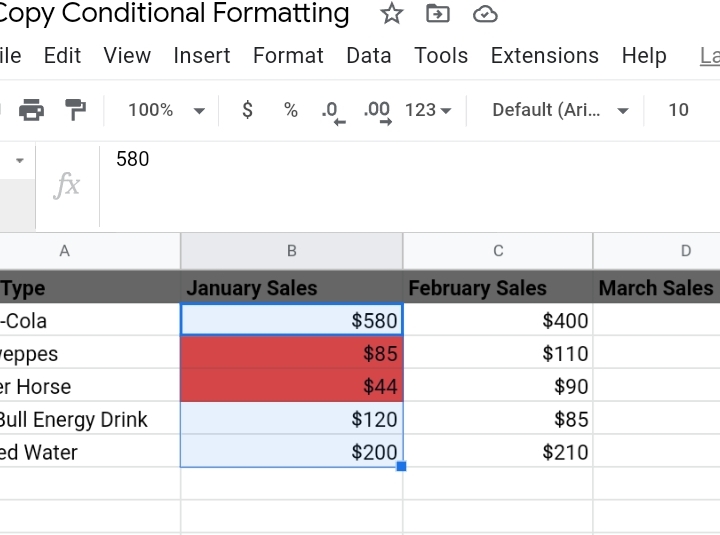
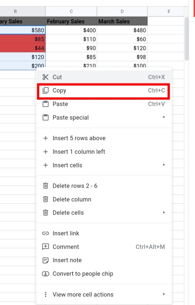
Step 2: Right-click on the cell and select Copy or press the control key + C on your keyboard.
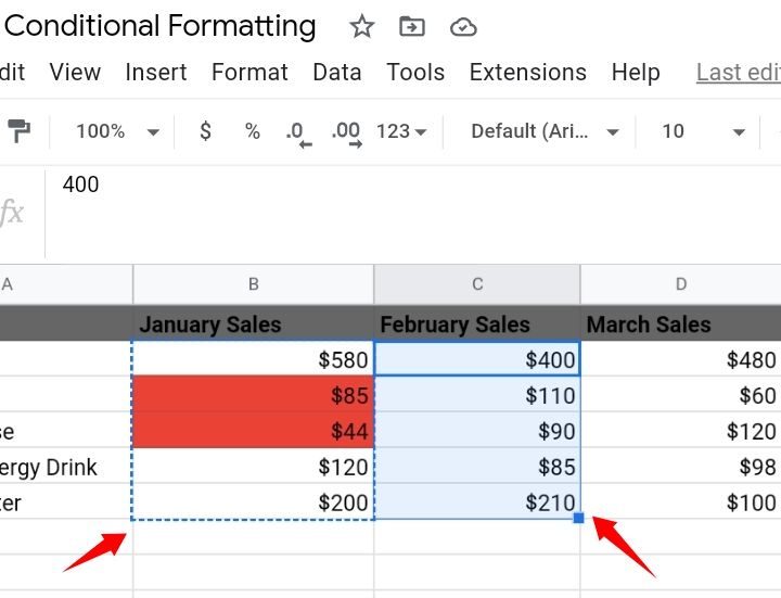
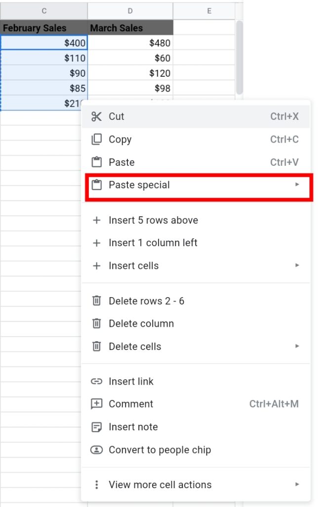
Step 3: The borderlines of the copied cells are replaced with short blue dashes which means the format has been copied successfully. Highlight all the cells in column C.
Step 4: Right-click on the column. A drop-down menu is displayed. Select Paste Special.
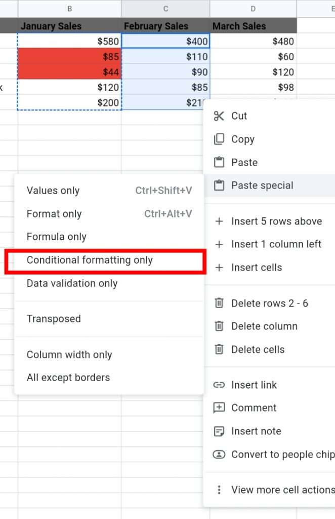
Step 5: Other options are produced. Select Paste Conditional formatting only.
Step 6: The values less than a hundred dollars are highlighted in red.
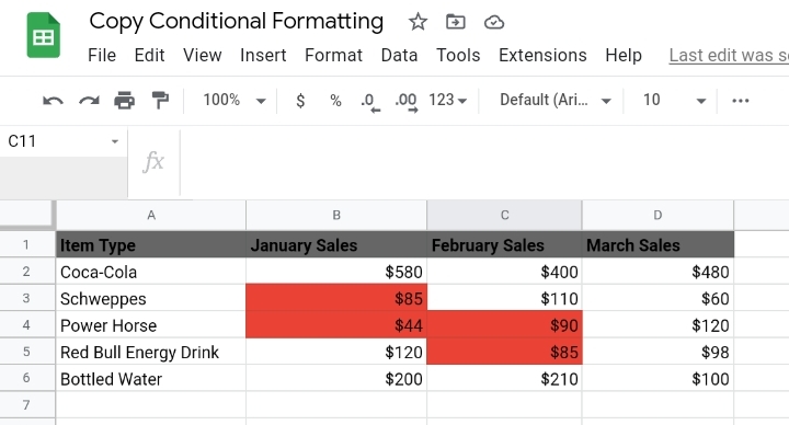
You can repeat the process for other columns in the worksheet
Method 2: Copy Conditional Formatting via Paint Tool
Another means of copying conditional formatting is with the Paint tool. The Paint tool copies texts in cells and pastes them to the selected cell or range of cells.
Step 1: Select a cell in column B which has the conditional format applied to it.
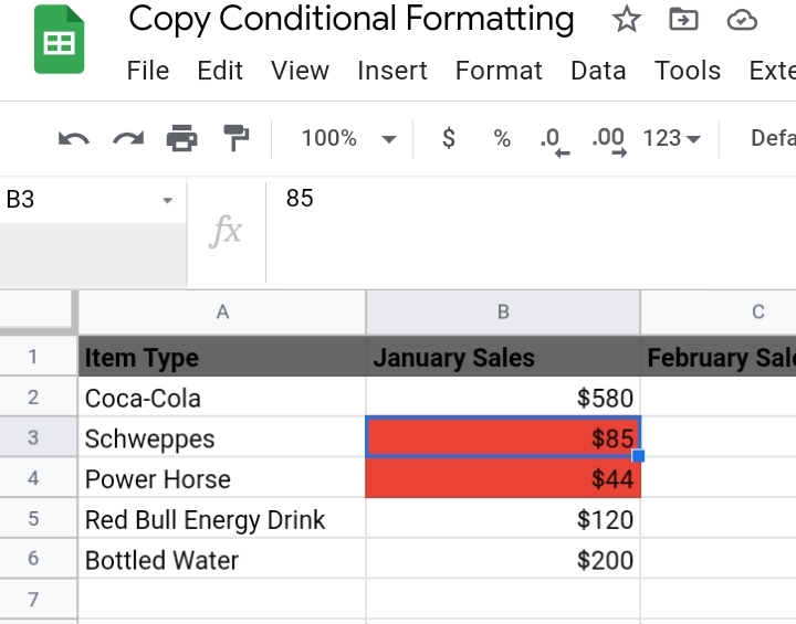
Step 2: On the top left of the toolbar, there is an icon that looks like a rolling painting brush. This icon represents the paint tool. Click on it. The icon turns green which means it is activated and ready to go.
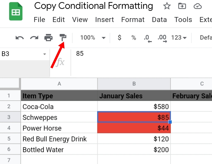
Step 3: The selected cell’s borderlines are replaced with short blue dashes which indicates the format has been copied.
Step 4: Highlight the cells in column C by using the drag and drop method or by clicking on the box icon displayed.
Step 5: Select Paste format only.
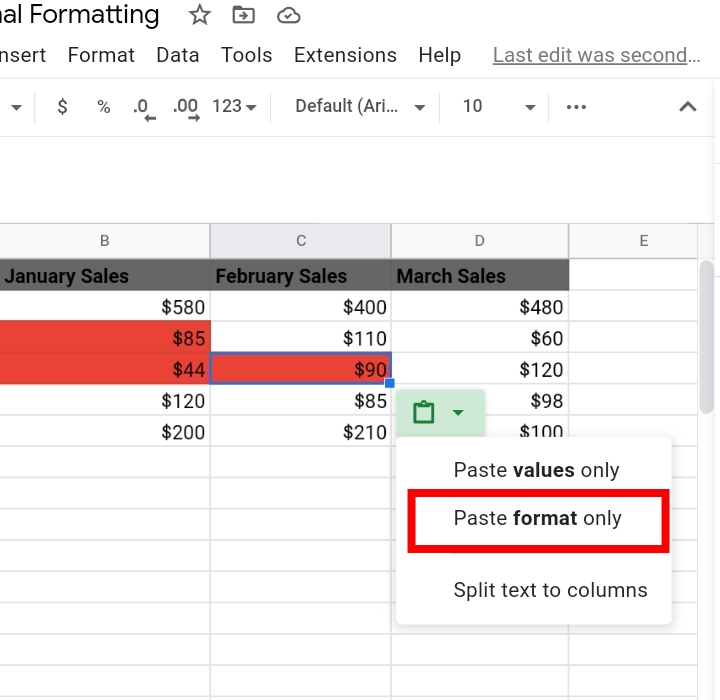
Step 6: The sales in column C become highlighted which means they are formatted.
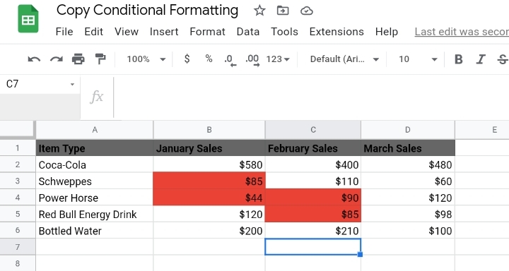
Method 3: Duplicate the Formatting Rule
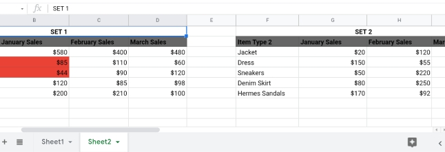
This technique is employed when you have two sets of different information on the worksheet. In the sample below, we have the first set of data from column A to column E and the other set from column G to column I.
The second set doesn’t have conditional formatting placed on it yet, so we are going to duplicate the conditional format placed on the first set and edit the range to suit the second set of data.
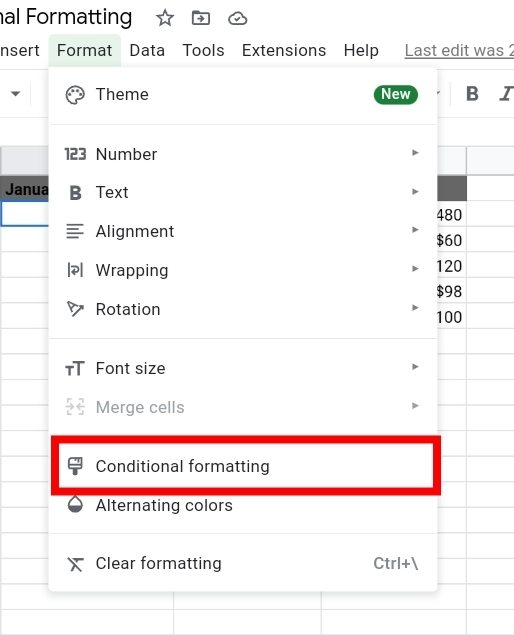
Step 1: Click on Format on the toolbar.

Step 2: Select Conditional Formatting.
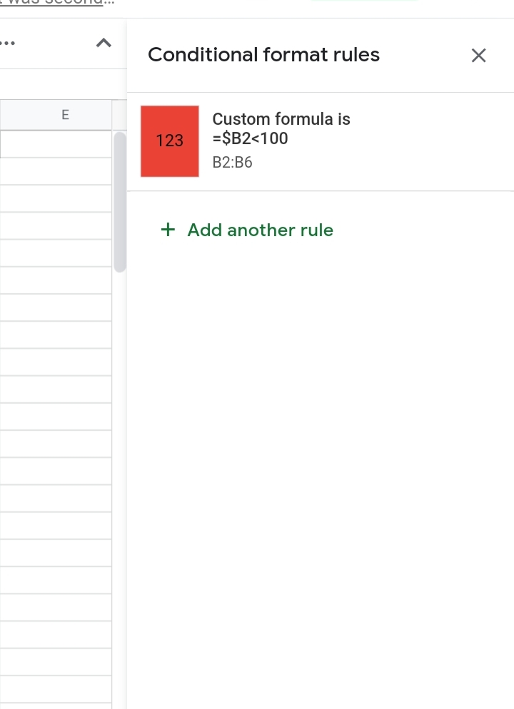
Step 3: A tab is opened on the right side of the worksheet. Select Add another rule.
Step 4: Create a duplicate of the first rule but adjust the cell range to that of the first column in the second set of data that is G3:G7
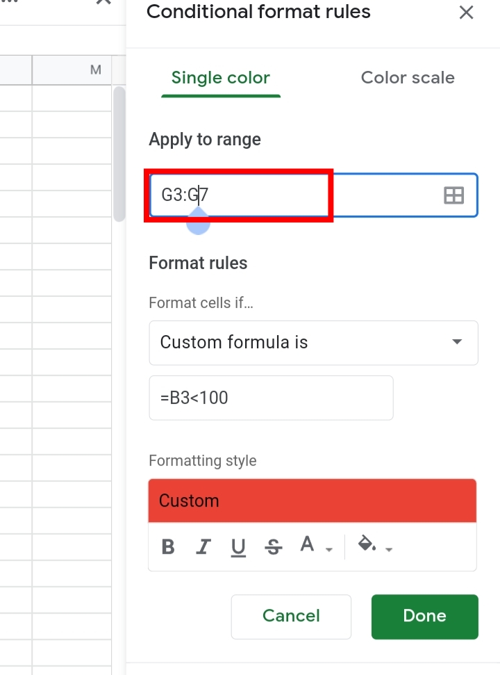
Step 5: Click Done. The two rules are placed on the same worksheet and the cells that fit the set condition are highlighted.
Method 4: Expand The Range of the Rule
If you don’t like the copy and paste method stated previously, you can simply edit and expand the range of the cells on the rule.
Step 1: Click on Format on the toolbar.

Step 2: Select Conditional Formatting.

Step 3: A tab is opened on the right side of the worksheet. Select the rule there.
Step 4: Click on the grid box to add another range to the rule.
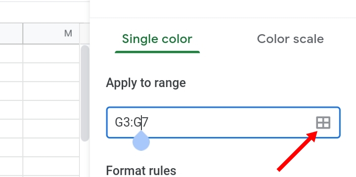
Step 5: In the box below the first range, input the second range or highlight the cells to automatically select the range, that is, C2:D6.
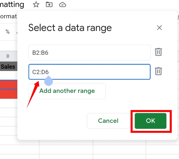
Step 6: Click on OK to save the additional range and Click Done. Now, the range of the rule is expanded. There are two ranges where the conditional format is applied in the worksheet.
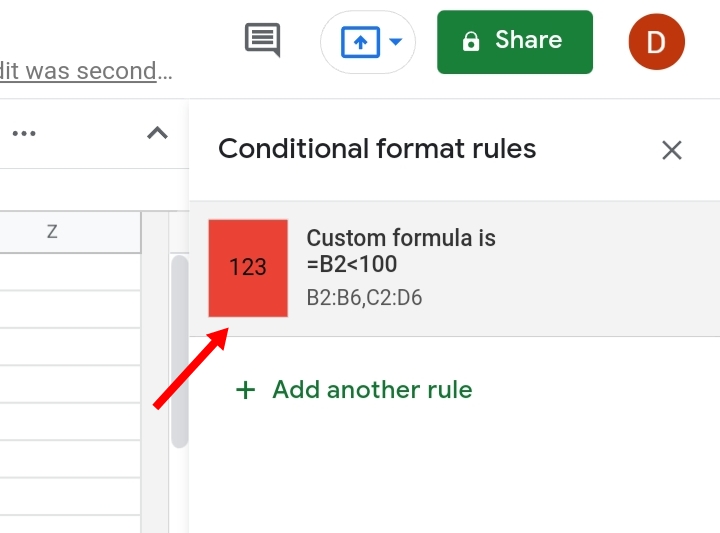
The conditional formatting is spread through the selected ranges.
How to Copy Conditional Formatting to Another Sheet in Google Sheets
Now, you know how to copy the format from one column to another, you need to know how to copy conditional formatting from one sheet to another.
Step 1: On the title of the sheet below, click on the dropdown arrow here.
Step 2: A menu is displayed. Click on Copy.

Step 3: Two options are produced, each asking if you want to copy to a new sheet or an existing sheet. Select Existing spreadsheet.
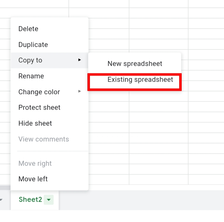
Step 4: A tab is opened, asking which document you want to paste the spreadsheet into.

Step 5: Select another document and click select.

A pop up is displayed indicating that the copied sheet has been pasted into the selected document along with the conditional format.

Closing Thoughts
Now, you know How To Copy Conditional Formatting in Google Sheets using 4 different methods in 2022.
Conditional formatting is a very significant tool that makes reading more concise and easy to understand. I hope you found this guide helpful. Thank you for reading.


