Anyone inputting data into a worksheet is bound to make mistakes at some point, especially when inputting large sets of data.
This technique is used to identify differences, similarities, duplicates between rows or cells in a column. It is very easy and quick to do, and it is sure to produce accurate results.
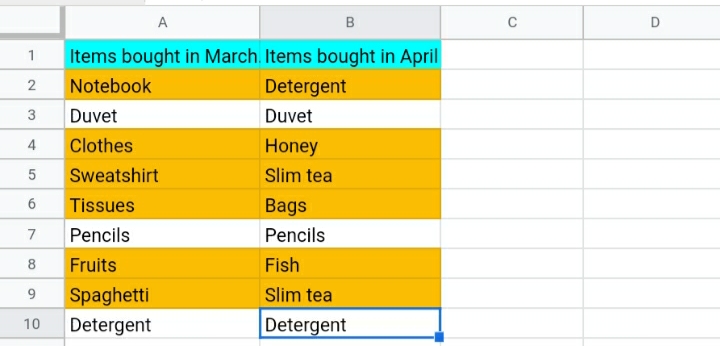
For the tutorial, we will be using a Google sheet consisting of two columns. Column A represents Items bought In March while Column B represents the Items bought in April. We compare with them in different way.
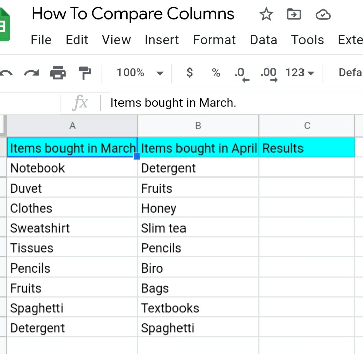
How to Compare Two Columns for Exact Row Matches.
This is the fastest and easiest way. It is also called cell-by-cell comparison. Your google sheet needs to point out which row has the exact or diverse data in a column and display the results.
We would simply construct a fresh column for the results and show TRUE if the set of data in the cell match and FALSE if they don’t match.
The formula used for comparing the columns is:
=A2=B2
When this formula is used, it produces a result of either true or false in Column C to show if the two columns match or not.
This technique is done in brief and quick steps.
Step 1: Input the formula above =A2=B2 in the function fx tab.
Step 2: Click Enter.
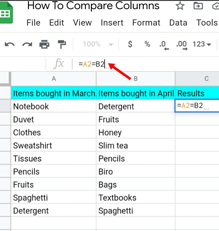
Step 3: A TRUE or FALSE statement is displayed in column C for results.
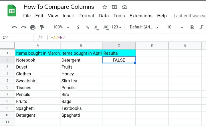
Step 4: Click on the other rows in column B. The effects of comparing columns A and B will be displayed in column C.
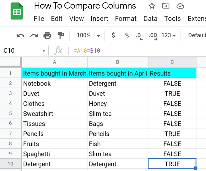
How to Compare Two Columns and Show Meaningful Text.
This technique is used when you are not the only person who is working on that particular google sheets. A third party viewing your worksheet might not comprehend what True or False means on the Google sheet.
This is where you provide more explanation of the outcomes in column C. For example, instead of displaying True Or False, you can replace them with MATCH for row items that match and NOT MATCHING for row data that do not match.
We would utilize the formula: =IF(A2=B2,”Matching,Not Matching”)
Step 1: Input the formula =IF(A2=B2, “Matching,Not Matching”).in the formula in the function section at the top of the google sheets.
Step 2: Click Enter on your keyboard.
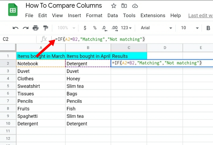
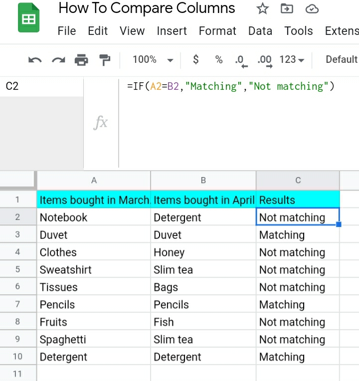
Step 3: The TRUE or FALSE statement is now replaced with MATCHING or NOT MATCHING as the results of the similarities between the second rows in column A and column B.
Step 4: Click on the other rows in column B. The outcomes of comparing the two columns will be displayed as MATCHING or NOT matching in column C.
How To Compare Two Columns to Find Matching Data.
The previous topics provided steps mainly on how to find out if the data in the cells in the columns are matching or not and if you want to compare two columns and find out which data in column A are repeated in column B and vice versa.
This technique is used to check for duplicates in a given set of data. Here, we use Conditional Formatting to find duplicate data in your google sheets. Conditional Formatting is a method used to format cells in your worksheet based on a set condition. It is done in the steps listed below.
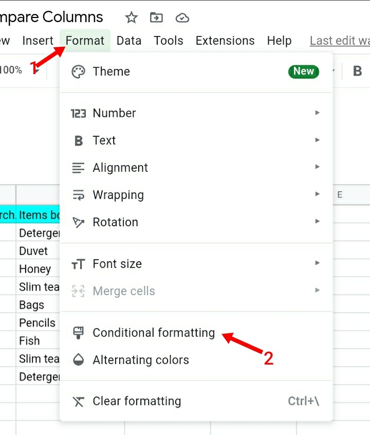
Step 1: Click Format on the tab section.
Step 2: From the list of options, select Conditional Formatting.
Step 3: A conditional formatting rules sidebar is displayed on the right-hand side of the google sheets.

Step 4: Type in the range of cells you want to apply the formatting on, in the box below Apply to range as shown below. In this example, we want to see the highlights of column A only. So we type A2:A12.
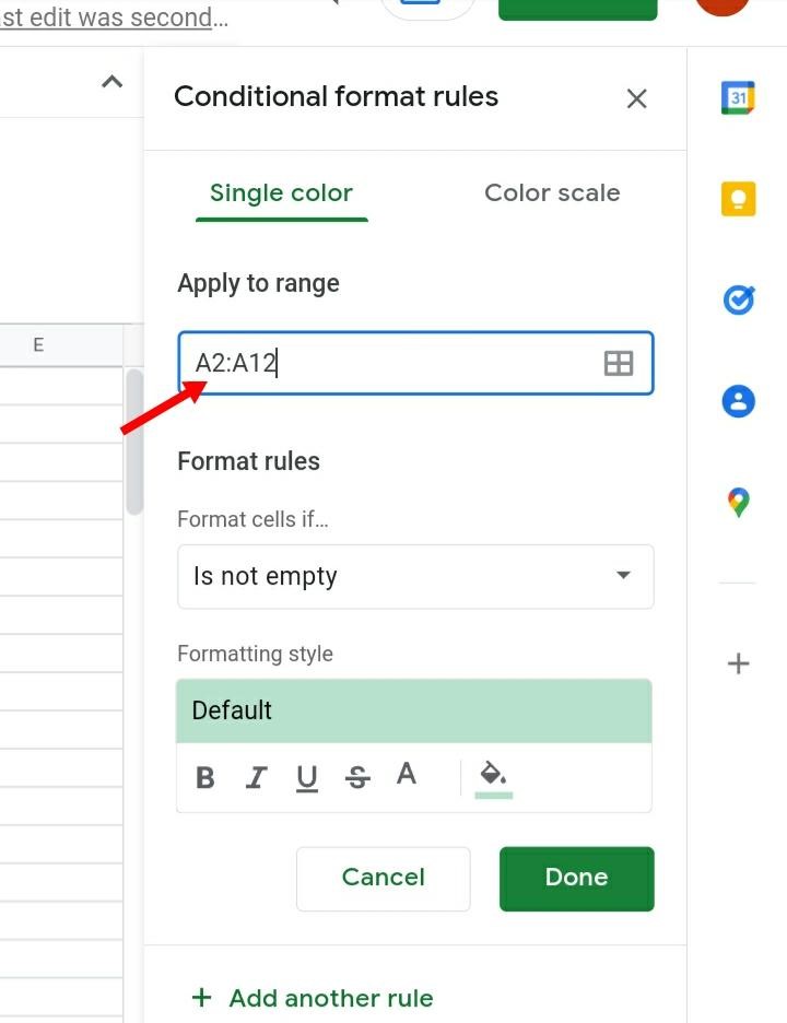
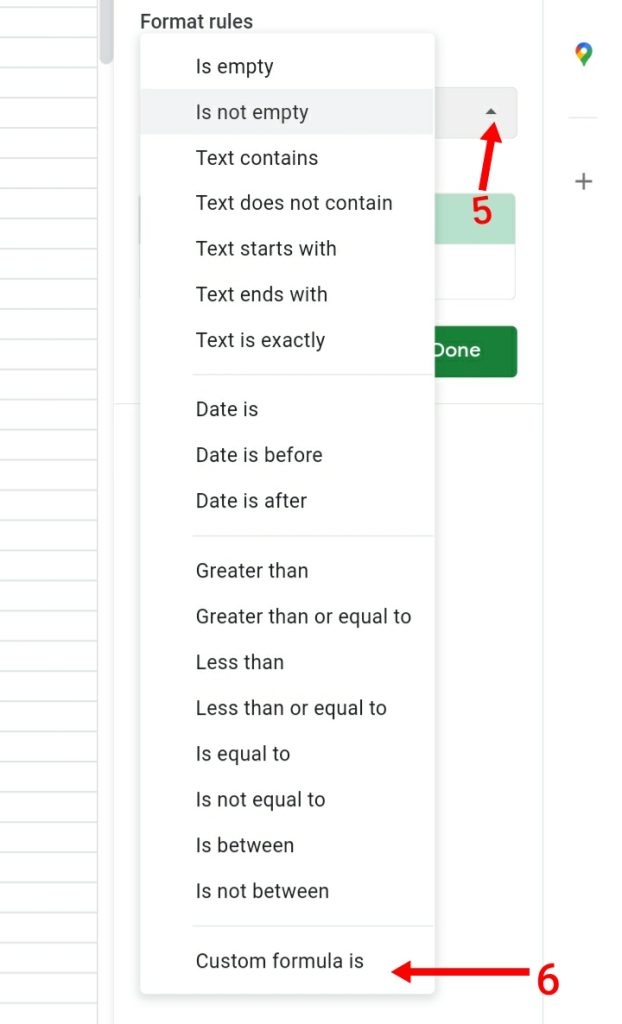
Step 5: Under the format rules tab, Format Cells If, select the arrow.
Step 6: Click on Custom Formula is on the menu.

Step 7: Enter your custom formula there. The formula is =COUNTIF($A$2:$A$10, B2)>0. Click on Done.
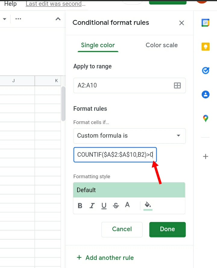
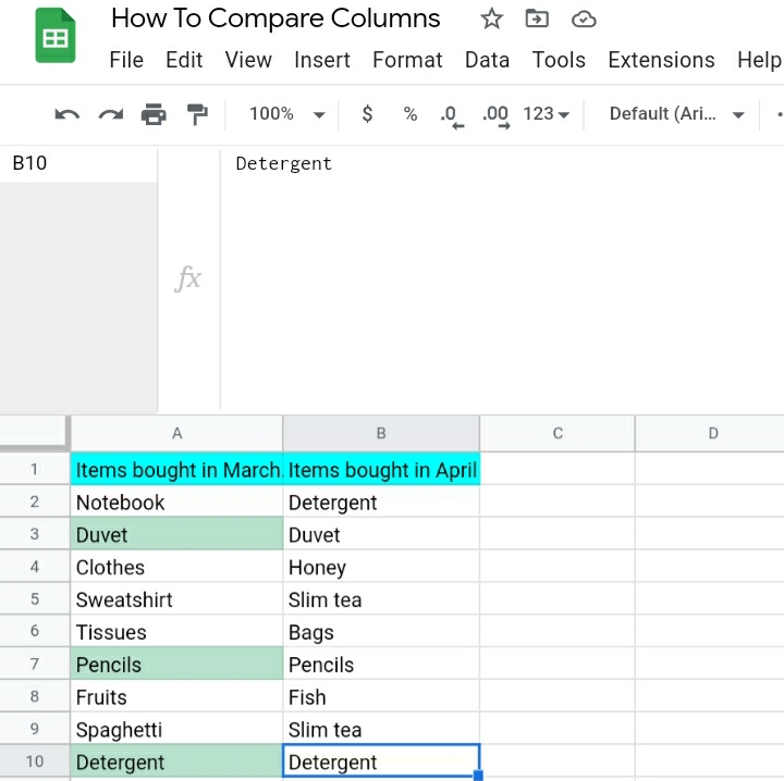
You would see all matching data present in the two columns highlighted with a default color. The next topic will explain how we can change the default highlight color to the color of your choice.
How To Compare Two Columns and Highlight Matching Rows.
If instead of displaying results in a separate column, you would rather have rows with matching data, highlighted in your color of choice, then you can perform Conditional Formatting.
Step 1: Click Format from the tab section.
Step 2: Click on the Conditional Formatting section.

Step 3: The conditional formatting rules section opens at the right-hand side of the google sheets.

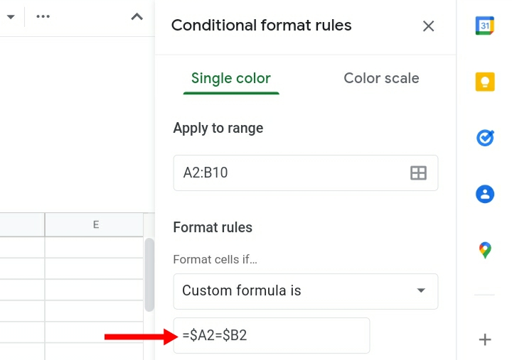
Step 4: Input the range of cells in the column you want to be compared under Apply to range. We input A2:B10.

Step 5: In the Format rules section, ” Format cells if”, click on it.
Step 6: From the menu that is displayed, Click on Custom Formula is.
Step 7: Input Value or Custom formula: =$A2=$B2.
Step 8: Click on Formatting style.
Step 9: Select the Fill Color Icon. Pick the color you want to use. The selected color shows matching cells or rows.
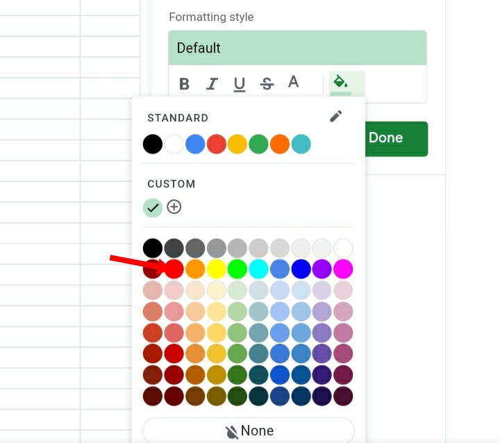
I chose Red for the highlights for the matching rows or cells.
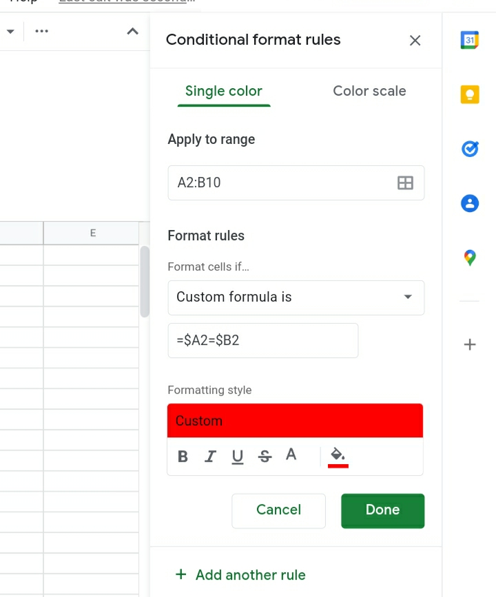
Step 10: Click on Done.
You would notice all matching cells in the two columns are highlighted in the color picked.
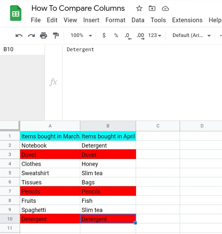
NOTE: In case you want to only highlight rows or cells that DO NOT match. You would change the formula used in Step 7 to =$A2<>$B2.
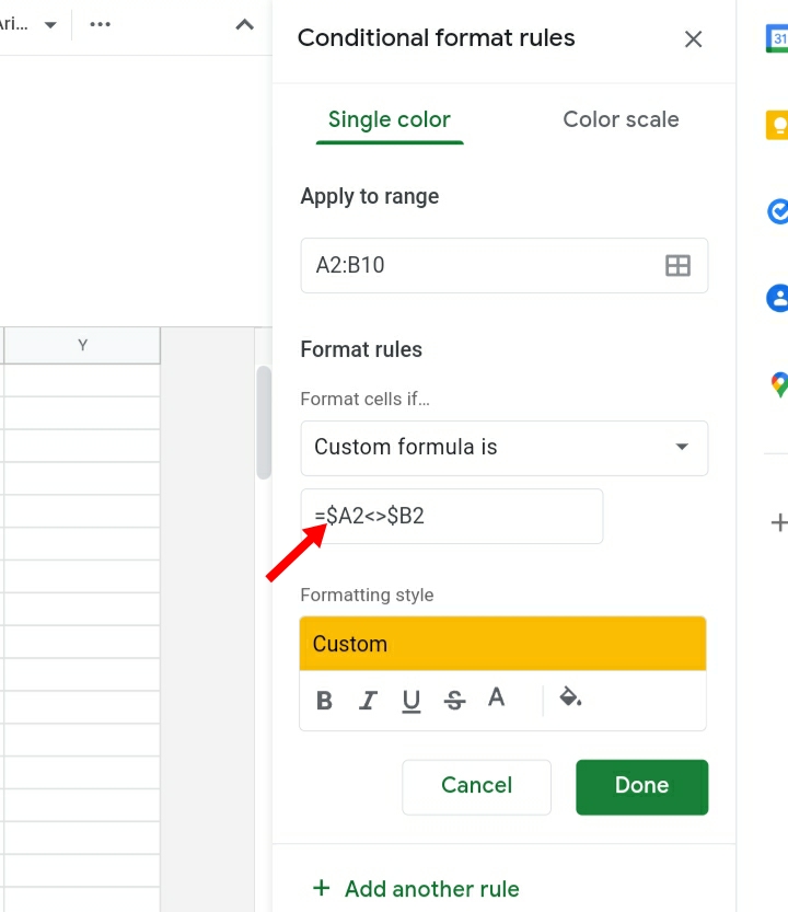
If you followed the steps correctly, the rows of data in each column that don’t match would be highlighted in the color picked as shown below:
How To Compare Two Columns and Find Missing Data.
This technique is used to find data present in column B but not in column A and vice versa.
It is easily done with the previous steps taken in Topic 4 except step 7 has a different formula.
Step 1: Click Format from the tab section.
Step 2: Select the Conditional Formatting section.

Step 3: The conditional formatting rules section opens at the right-hand side of the google sheets.
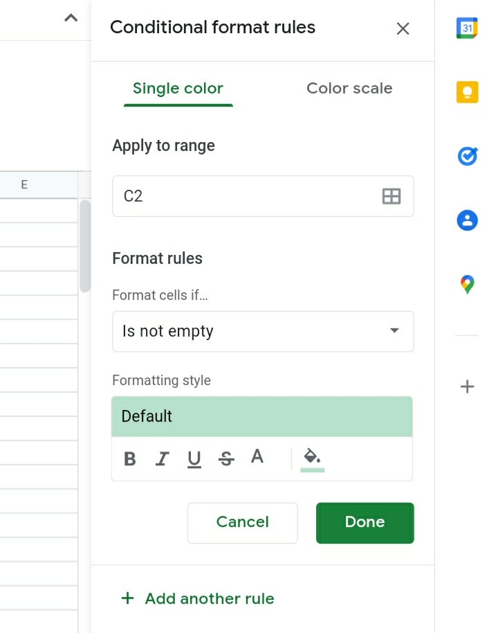
Step 4: Under Apply to range, input the range of cells in the column you want to be compared. We input A2:B10.
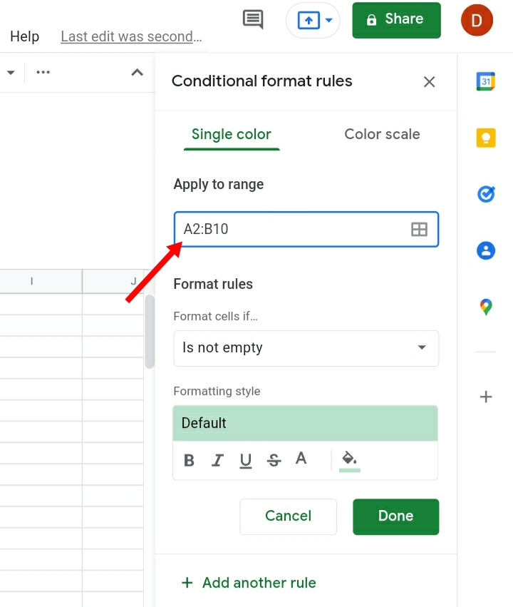
Step 5: In the Format rules section, ” Format cells if”, click on it.
Step 6: From the menu that is displayed, Select Custom Formula is.

Step 7: Input the custom value as =COUNTIF($A$2:$A$10, B2)=0.
This formula shows the number of occurrences of data in column B present in column A.
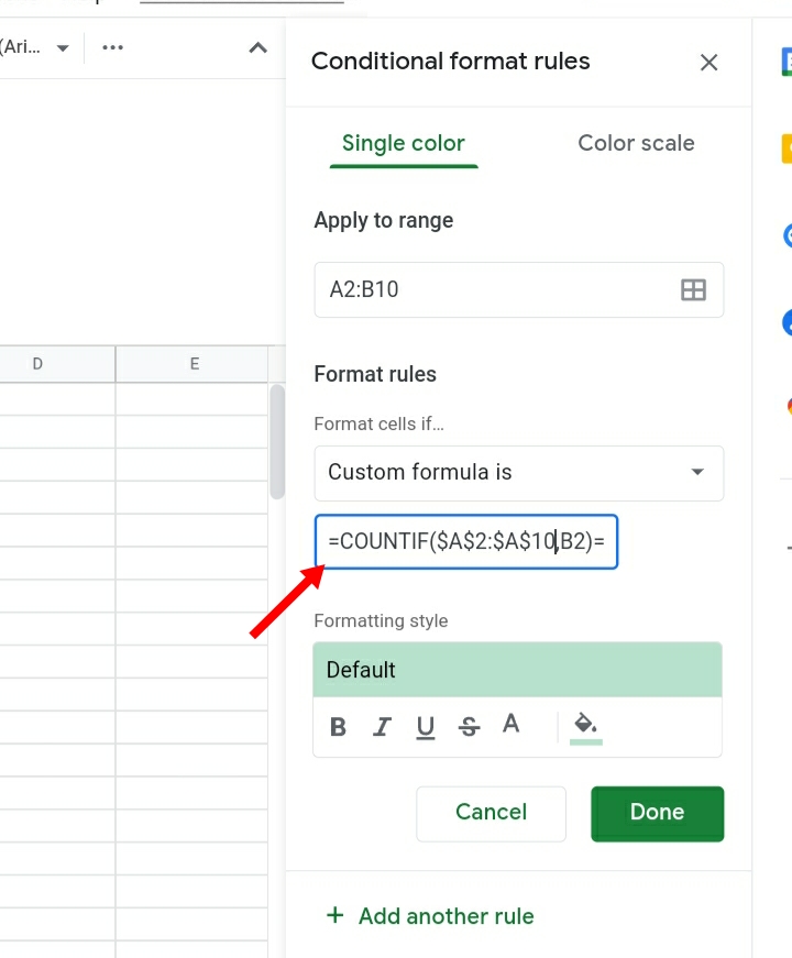
Step 8: Click on the Formatting style
Step 9: Click on the Fill Color Icon. Select the color you want to use. The selected color shows matching cells or rows.
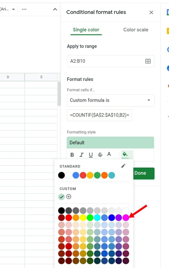
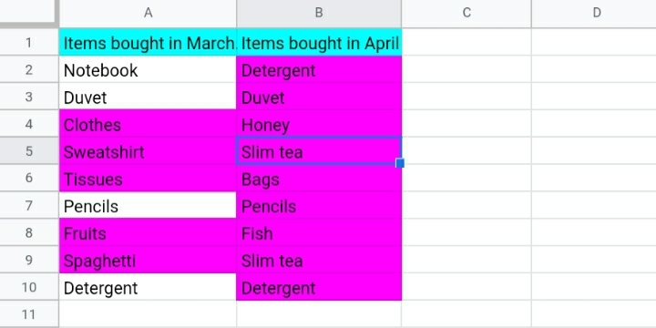
We picked the Purple color to emphasize the missing rows in the two columns.
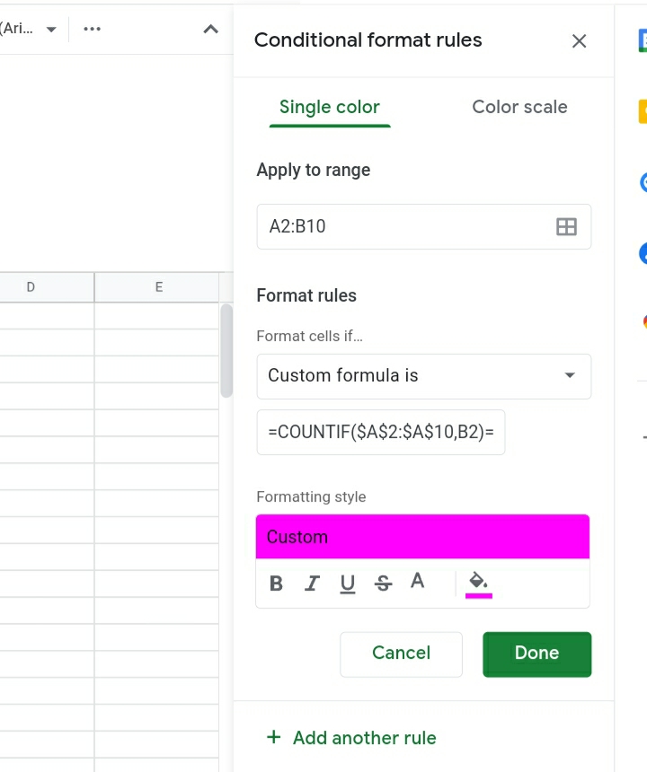
Step 10: Click on Done. The rows of data in column A that are missing in B are highlighted and vice versa.
Final Thoughts:
This guide was made to help people who find this tool in Google sheets difficult to operate and understand.
These techniques are very useful when comparing long and large sets of data in cells and columns. We hope this tutorial is helpful. Thank you.


