The analysis of stocks and its continuously changing nature can be a little hard to follow. In most cases, the prices are affected by random trends; the sudden rise or drop in prices is not always an indication of how well a certain market is doing.
Studying past data is crucial for future decisions. This can happen through studying the Moving Average of companies, as it indicates the patterns of closed prices movement.
In the following article we will provide a tutorial for Calculating the Simple Moving Average in Google Sheets for one or more assets in a certain period of time.
What is the Simple Moving Average (SMA)?
The Simple Moving Average is simply the average price of a stock. It can be used for predicting future trends of an increase or decrease in prices.
Calculating the average rules out the random fluctuation in data, and thus gives a clear view of one or more markets. It is called “moving” because it is being continuously updated.
The Moving Average differs from the Simple Moving Average in regard to the covered period of time.
Wherein the Moving Average calculates time in years, the Simple Moving Average calculates time in a handful of days, or months. A SMA of a 10 day period, for example, is called a 10-day SMA.
If we were to cover an SMA of a 20 day period, it would be called a 20-day SMA, and so forth. In the following tutorial we will be discussing the latter type.
How to Calculate Moving Average in Google Sheets
The GOOGLEFINANCE Function can be used within Google Sheets. It extracts data from Google Finance and implements it directly into the sheet.
This is your closed prices stock data, this is the data you will be using to then calculate an average using the AVERAGE Function in Google Sheets.
Let’s break down each of the two functions, GOOGLEFINANCE, and AVERAGE, learn how to perform both, and then use them together to reach the desired SMA.
The GOOGLEFINANCE Function
Google Finance provides real-time market quotes, the exchanges made internationally, updated financial news, and overall analytics to help you make well informed trading decisions.
The function GOOGLEFINANCE itself provides stock data, historical and news, from the website and directly into your Google Sheets.
The function is as follows:
GOOGLEFINANCE(ticker, [attribute], [start_date], [end_date|num_days], [interval])
Let’s break it down to understand each segment:
- The ticker is the symbol or initial letters corresponding to your desired stock. It can be written as either both the exchange symbol and the ticker symbol as in: “NASDAQ:TWTR”, where “TWTR” represents Twitter, or by sticking to the ticker on its own: “TWTR”.
- The attribute is the value that you seek and want to access from the ticker you provided. To access the prices, use the attribute: “price”. Other values could be: “high”, “low”, “volume”, etc. If not specified, the default attribute fetched will be “price”.
- The start-date is the date from where you want the data fetching to start.
- The end-date, in the same sense, is the date from where you want the data fetching to end.
- The num_days is the value or amount of days you want data fetched from. You can either use an end date, or specify the amount of days you want.
- The interval is the frequency of your fetched data. You can fetch “daily” or “weekly” data.
Note: it is important to understand the elements of the function as you will most likely have to write it manually to activate it. I.e: Copy and Paste usually does not work.
So, to fetch data using the GOOGLEFINANCE Function for Twitter stock prices, select a blank cell in Google Sheets and write the following formula:
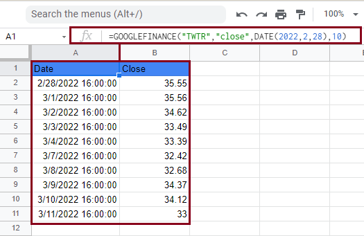
=GOOGLEFINANCE(“TWTR”,“close”,DATE(2022,2,28),10)
The above function fetches the closed prices for TWTR from the date (02,28,2022) and up to 10 days after that. The function and the fetched data should look like this:
The AVERAGE Function
This function simply calculates the mathematical average of the set of values you select. This function is written as follows:
=AVERAGE(value1, [value2, …])
Broken down to:
- value1 is the first value taken into calculations of the AVERAGE function.
- value2 is the second value taken into calculations of the AVERAGE function.
This can go on for as many values as you want. For larger calculations, this can be time consuming, so it is recommended that you use the “cell:cell” type of format.
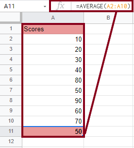
So, for example, if we have a set of values that we want to calculate the average of, we will select the first blank cell under the last value, and write the following formula:
=AVERAGE(A2:A10)
This should give you the following result:
How to Calculate Moving Average in Google Sheets Using a Formula with GOOGLEFINANCE and AVERAGE Functions
Now that we have learned how each of the functions (GOOGLEFINANCE and AVERAGE) works separately, we will now see how they work together.
On a larger scale now, let’s say you want to calculate the 3-day SMA of Twitter stocks over the last month. The first step would be fetching data of 30 days prior to today’s date. We can do this through the following formula:
=GOOGLEFINANCE(“TWTR,”close”,TODAY()-30,TODAY())
Let’s break down the new parts,
The today() segment automatically fetches today’s date, today()-3o inserts the duration of 3o days prior to today’s date. If we were to fetch 15 days prior to today’s date, this segment will be written as today()-15 and so forth.
Select a blank cell and write the above formula. This should retrieve the stock prices of Twitter over the last 30 days and it should look like this:
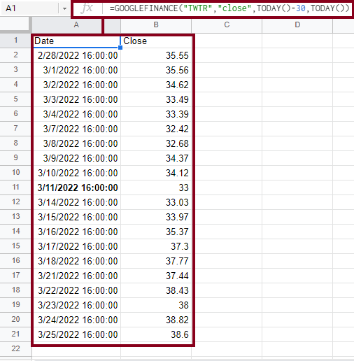
You might notice that the retrieved data fills up to cell 21 while the requested data was for 30 days. This is because data is only recorded during trade days, all off-days are not counted and therefore return no data.
Now to calculate the 3-day SMA, head over to the fourth cell in column C, which we will dedicate to the AVERAGE formula and results. In the blank cell, write the following formula:
=AVERAGE(B2:B4)
By pressing the Enter or Return key, you should have the calculated average of the first three days in place as shown below:
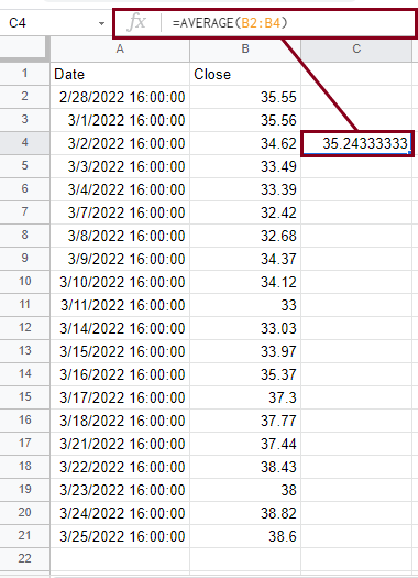
Now we have the 3-day SMA of dates 28/02/2022 through 2/3/2022. Now if we want to calculate the 3-day SMA from the subsequent days of each date, and everyday that follows, we would have to write the above formula for each three subsequent cells.
Doing this for each cell is tiresome and time-consuming. A much easier way to apply the above formula on all of your data is by selecting the main cell in which the main formula is written (cell C4) and dragging down from the corner to cover the rest of the cells.
Or simply by using the shortcut ctrl+enter (sometimes prompted by Google Sheets) this auto-fills the formula into the rest of your cells.
Now your data should look like this:
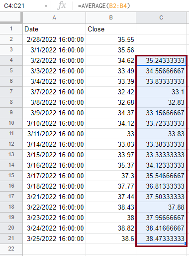
An overall breakdown: Column A displays the dates of the trade days over the last 3o days. Column B displays the closing prices of each day.
Each cell in Column C displays the average of the past 3 days, and an overall look on the column shows the 3-day moving average of your data.
How to Calculate Moving Average in Google Sheets Using a Formula with GOOGLEFINANCE and QUERY Functions
Now that you have mastered the above combination of functions, you might want to expand your analysis to cover not only one asset, but two, three, or way more than that.
By strictly following the above steps, you will get results, but you will also get an overcrowded worksheet, a mayhem of numbers and dates, and a difficulty in comprehending any data at all.
This issue is best solved using the QUERY Function. It gives you the chance to view SMA of a given number of days prior to the current day.
It is a dynamic formula that is always updated, and will directly show the SMA of many assets at the same time, to make comparisons and analysis more clearer and much simpler.
For this part of the tutorial we will be using 5 different assets and we will write them all in Column A in the following manner:
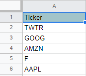
Let’s say that we will calculate a 5-day SMA of the previous assets, we will do so by using the following formula:
=AVERAGE(QUERY(GOOGLEFINANCE(A2,”close”,TODAY()-5,TODAY()),”Select Col2″))
Broken down:
(GOOGLEFINANCE(A2,”close”,TODAY()-5,TODAY())
- A2 is the cell in which our ticker is written. The start_date and end_date are presented as shown before using the TODAY()-5 method to fetch five days of data.
QUERY(GOOGLEFINANCE(A2,”close”,TODAY()-5,TODAY()),”Select Col2″)
- The QUERY function allows us to specify the exact data we want fetched. In this case, we want the closing prices which are in the second column, so we use “Select Col2” to achieve this.
AVERAGE(QUERY(GOOGLEFINANCE(A2,”close”,TODAY()-5,TODAY()),”Select Col2″))
- Since the QUERY Function only fetches the closing values, we want to calculate the SMA of these values so we use the AVERAGE Function to do so.
Now to apply all of this, select a blank cell in column B and insert the main formula from above. Drag down from the main cell to apply the formula to the rest of the sheet. It should look like this:

Conclusion
To sum up everything we have learned, we covered how to calculate the Simple Moving Average in Google Sheets using the GOOGLEFINANCE and AVERAGE Functions which is perfectly used when analyzing one or two different assets.
We also learned how to calculate SMA for multiple assets using the GOOGLEFINANCE and QUERY Functions. We broke down each formula so it would be easily understood and adapted to different inputs.
Hopefully, this was clear and easy to follow.


