Sometimes, when you are inputting different data types in a single worksheet, some texts are often misinterpreted as dates by Google Sheets.
For instance, you type in a text like 2-2020, which is supposedly a plain text but is misinterpreted as a date by Google. In this tutorial, we would show you How To Stop Google Sheets From Auto-Correcting Dates in 2022.
Stop Auto Formatting Numbers as Dates in Google Sheets
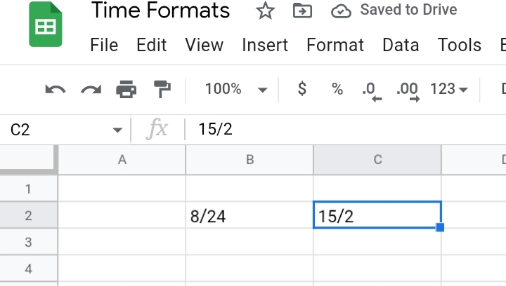
In the sample worksheet below, cell B2 has a text input that is 8/24. But when the text is entered, the value is changed to a date format.
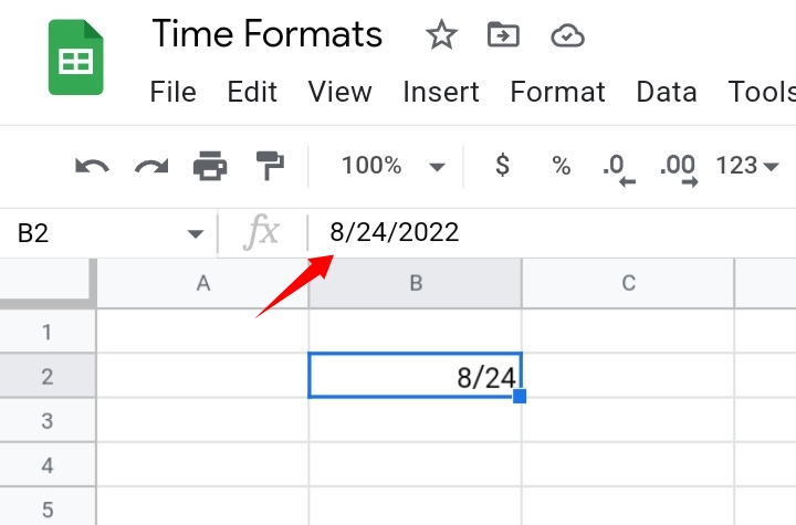
We want to prevent this from happening in two ways.
- Formatting value as plain text.
- Addition of an apostrophe.
Formatting Value as a Plain Text
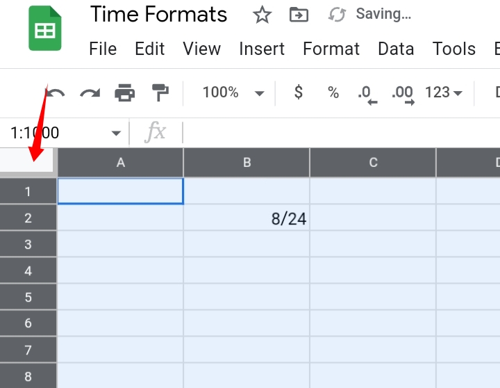
Step 1: Select the cell or column with the value. If the entire worksheet has similar values, highlight the sheet by clicking on the grey box at the top left corner of the worksheet.
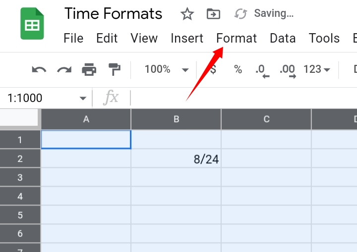
Step 2: Go to Format on the toolbar.
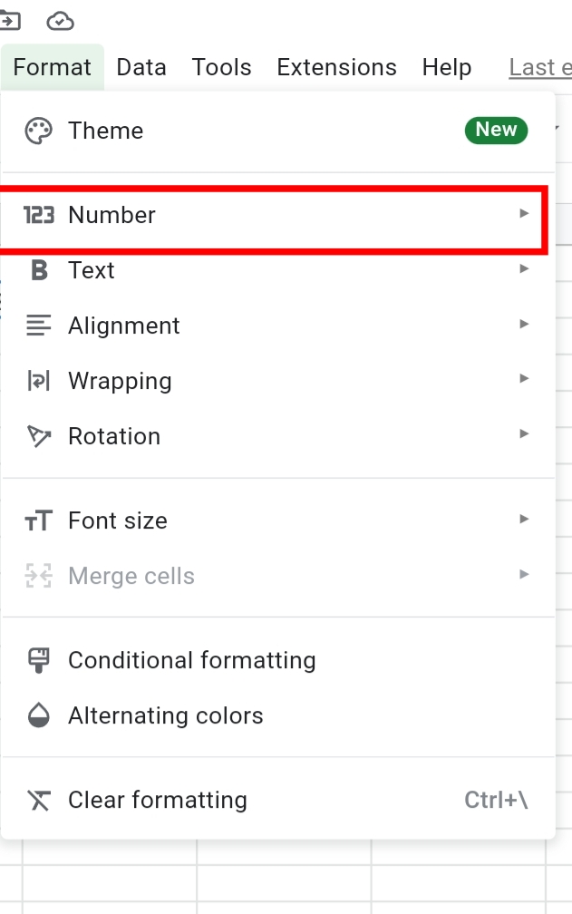
Step 3: From the drop-down menu, select Number.
Step 4: A list of options is displayed. Select Plain Text.
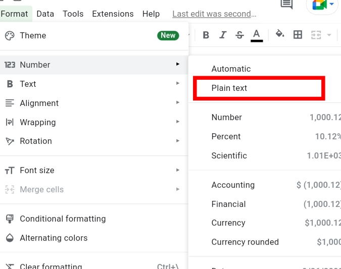
When this is done, the cells are formatted to plain texts so any value or digits entered would not be autocorrected as dates.
Addition of Apostrophe.
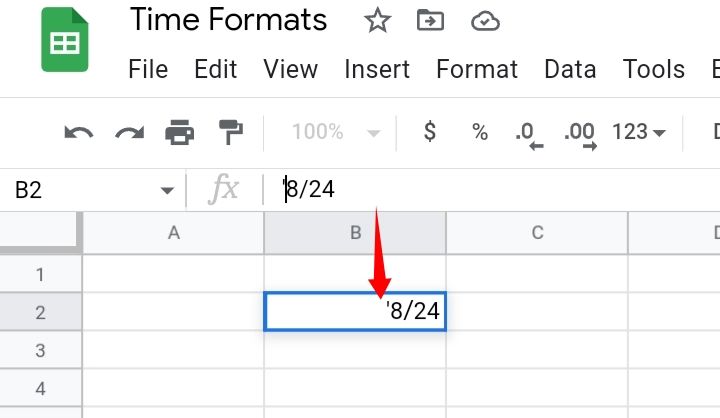
Another method used is the addition of an apostrophe (‘). The apostrophe is placed at the start of the value or before you enter the digits in the cell.
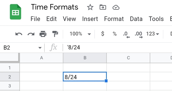
For example, the value 8/24 would be inputted as ‘8/24. When the digits are entered, the apostrophe is not displayed in the cell and the data remains unformatted.
How To Stop Google Sheets from Changing to Military Time.
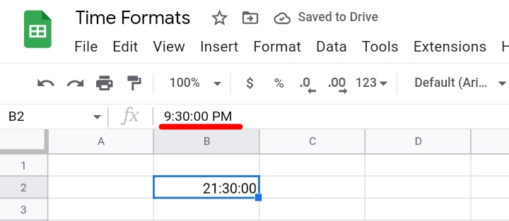
The default time format in Google Sheets is the Military Time format. But we would like to change it to the standard format commonly used on mobile devices, digital wristwatches, computers and so on.
Here, we are going to learn how to stop Google Sheets from automatically changing the time to the military time. There are two ways to stop it and we are going to highlight each method.
- Use of a function.
- Applying Custom Formatting.
Changing Military Time Format to Standard Time Format.
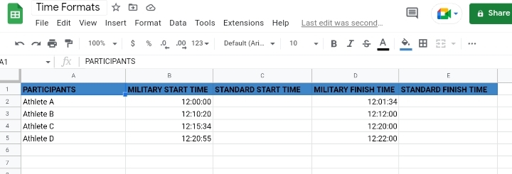
In the worksheet below is a stopwatch timing for the race tryout in a school. Each participant has a unique time spent covering a distance of hundred meters.
In the cell, B2 is the start time and in the cell D2 is the finish time. Athlete A runs the distance between 12:00:00 to 12:01:34. We want to convert the time into the standard time.
Use Of Function.
The function used takes the syntax below.
=TEXT(cell reference, “HH:MM:SS AM/PM”).
Where HH, MM and SS represent the hours, minutes and seconds respectively.
In our study case, we want to convert the start time in column B to standard time in column C. So, in cell C2, we enter the formula as
=TEXT(B2, “HH:MM:SS AM/PM”)
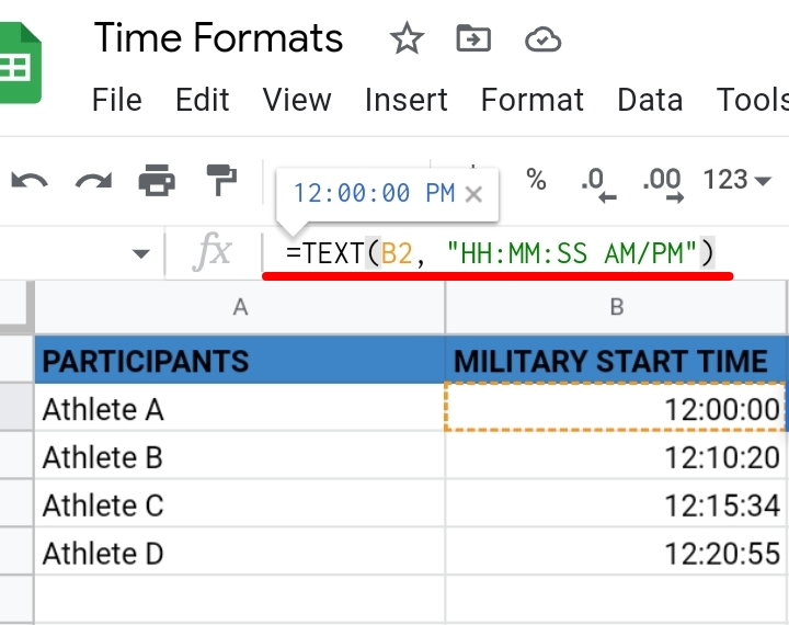
Press the Enter key and the time in cell C2 is displayed as 12:00:00 PM.
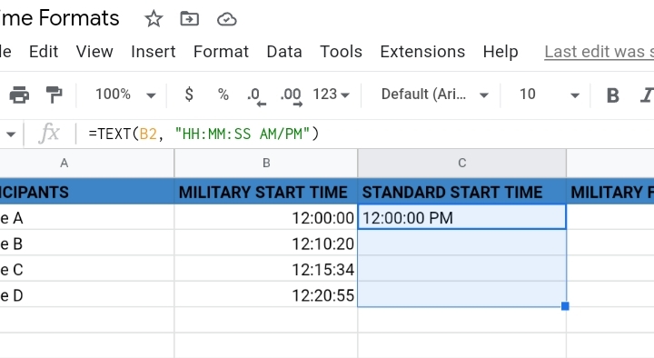
Drag down the formula into other cells to convert the times.
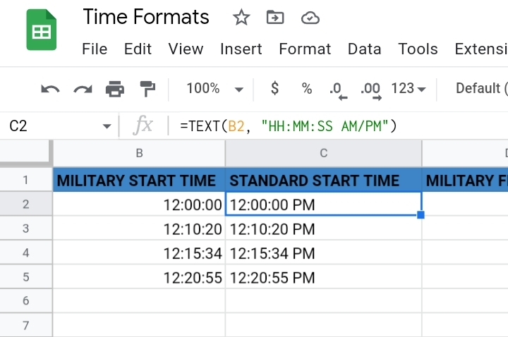
Note that this formula works because it is placed in another cell. It won’t work in the cell because the formula requires a cell reference. This is where the second method is most suitable for the conversion of time formats.
Applying Custom Formatting.
Step 1: Select the cells or range of cells you want formatted.
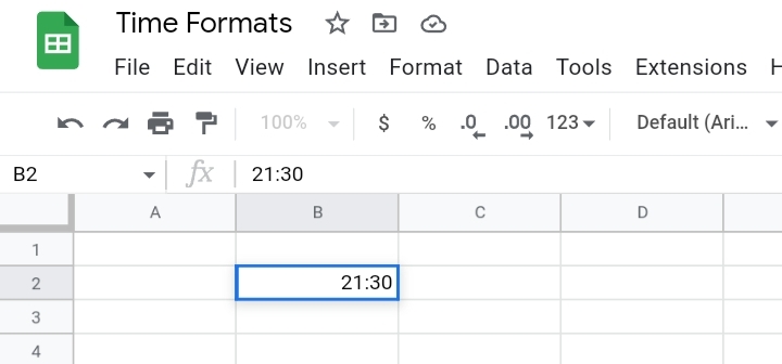
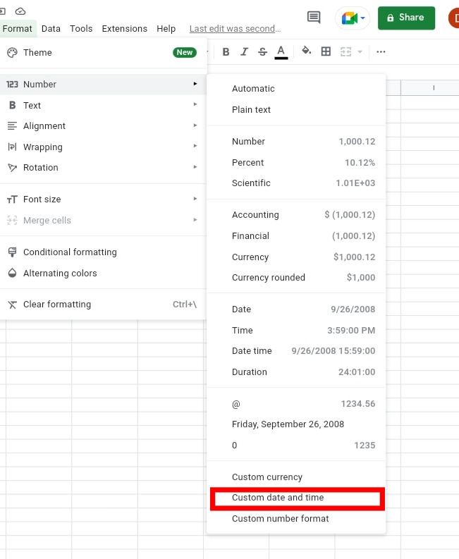
Step 2: Go to the toolbar and select Format.

Step 3: From the drop-down menu, select Number.

Step 4: From the new menu, click on Custom Date and Time.
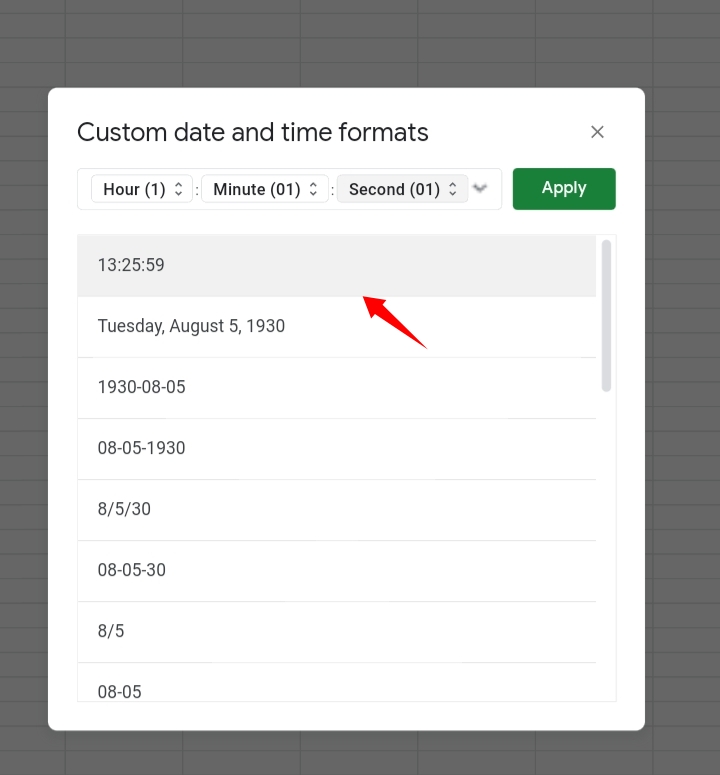
Step 5: In the opened tab, search and select the 12-hour time format. You can also add this manually into the textbox if you don’t have the format. (01:30:30 PM)
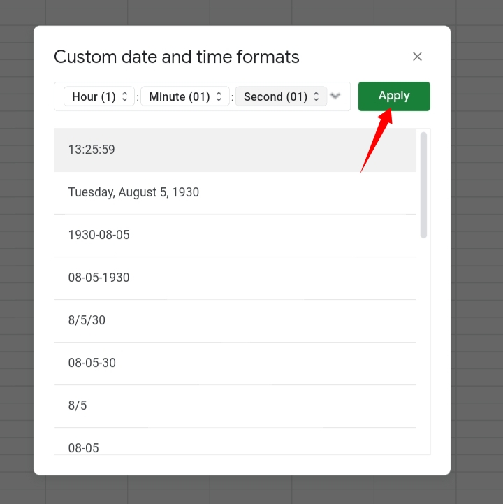
Step 6: Click Apply. The custom formatting is applied to the time in the selected cell range.
Final Thoughts.
As displayed above, the standard time format is a more suitable way of showing time on your worksheet. If you prefer the military time, you can keep the date as it is on your worksheet but do let us know which format you prefer personally in the comment section below.
Now you know How To Stop Google Sheets From Auto-Correcting Dates. I hope you found this useful. Thanks for reading.


