The randomize feature helps to sort out and shuffle texts and contents dynamically in a worksheet. In Google sheets, we can randomly sort and select the contents of a range of cells in more than one way.
This proves how versatile the randomize feature is. We are going to discuss How to Randomize a List in Google Sheets using three different methods in 2022.
How To Randomize a List in Google Sheets.
Shuffling texts and contents are very important especially when you’re trying to create a unique pair of two different texts. There are three methods used to randomize a list of any item on the worksheet. Using the list of names below, we would show you the three methods for randomizing ranges.
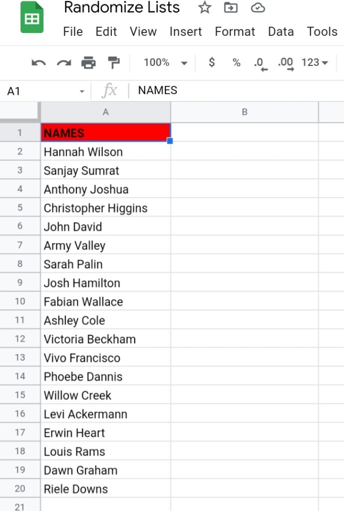
Method One: Using the Randomized Range Feature.
This is an inbuilt feature and doesn’t require any functions or formulas to operate. It is considered the fastest and easiest way of randomizing lists and it is done in a matter of seconds.
Step 1: Select the range of cells containing the names.
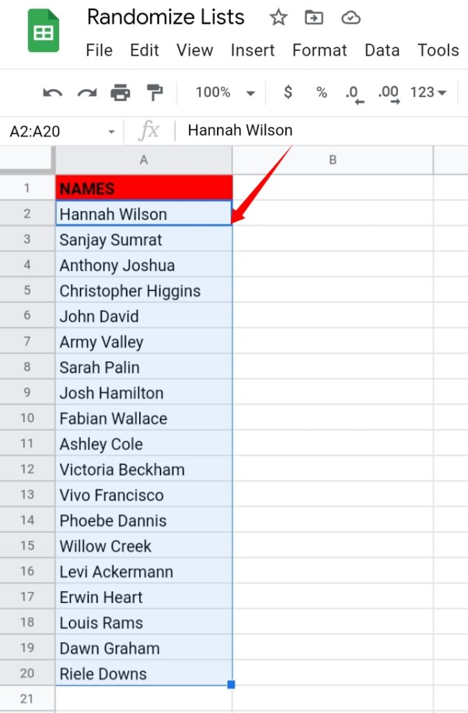
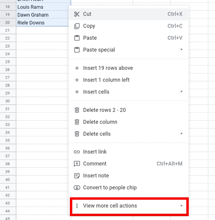
Step 2: Right-click on the range. A drop-down menu is produced. Select View more cell actions then select Randomize Range.
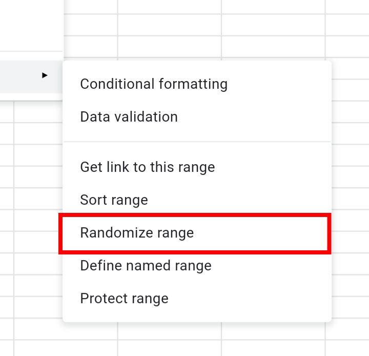
Step 3: The texts in the cells are shuffled randomly in the cells.
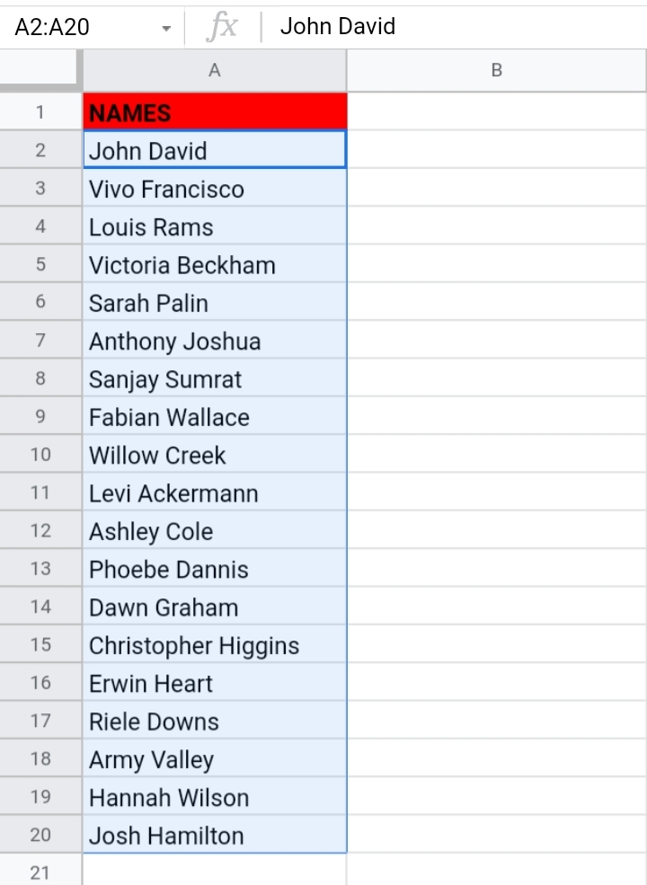
Alternatively, you can use the Data feature on the toolbar to randomize a list.
Step 1: Select Data on the toolbar.
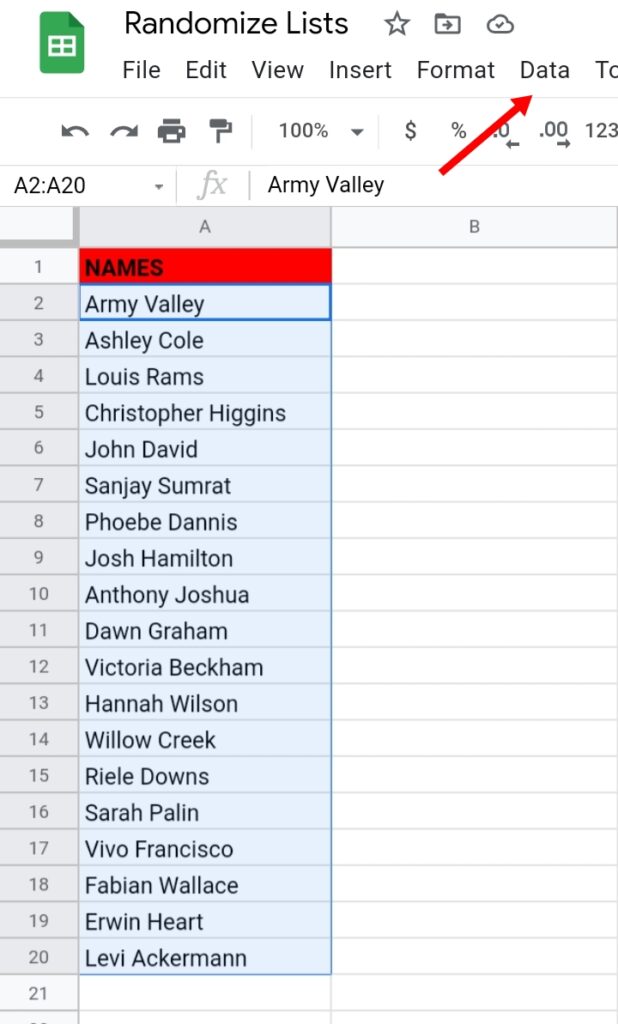
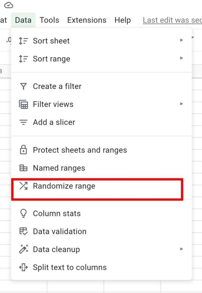
Step 2: From the drop-down list, select Randomize Range.
Step 3: The names in the cells switch and change positions in the column.

Method Two: How to Randomize a List using the SORT and FILTER functions.
This is a formal method used to randomly shuffle lists. This technique undergoes numerous stages which makes it a bit more difficult and longer than the first method.
Firstly, we use the RAND function to create and assign random numbers between zero and one, to each text in the worksheet. Then, we use the SORT and FILTER functions to randomize and arrange the list. This technique is quite versatile and can also be applied to similar applications like Microsoft Excel.
This is done in the steps stated below.
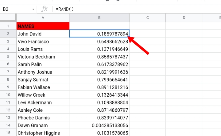
Step 1: In the blank cell B2, input the Formula =RAND(). Press Enter on the keyboard.
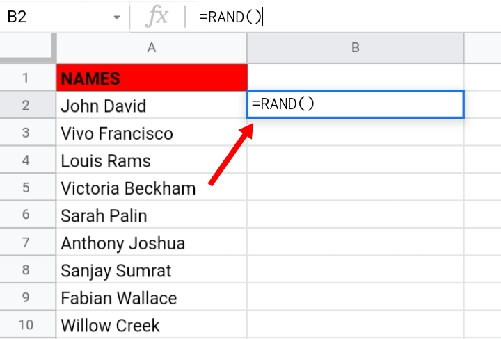
Step 2: As seen below, a random number in decimals is generated for the name in cell B2.
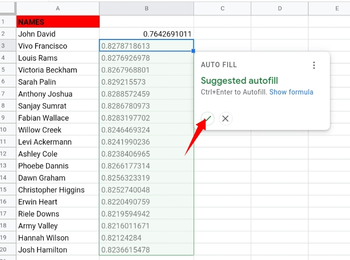
Step 3: Use the fill cube to copy and paste the formula into the remaining cells or by using the suggested autofill to automatically paste the random numbers for other cells in column B.
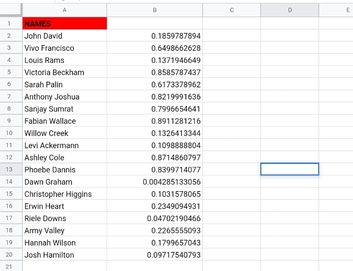
Step 4: Select any cell with a random number.
Step 5: Click on Data on the toolbar.
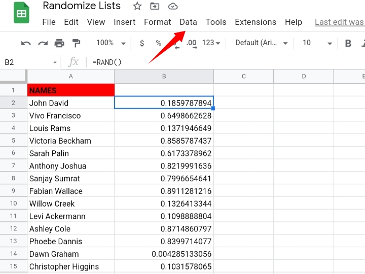
From the drop-down menu, select Sort Sheet. Then, Column B, (A to Z).
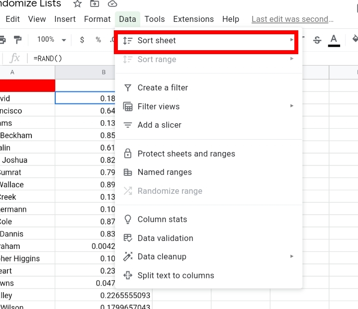
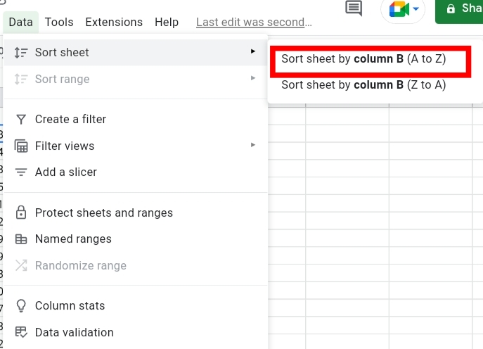
Step 6: Highlight column B which comprises the random numbers and press the Ctrl key + Delete or Ctrl key + Backspace on the keyboard to delete the column content.
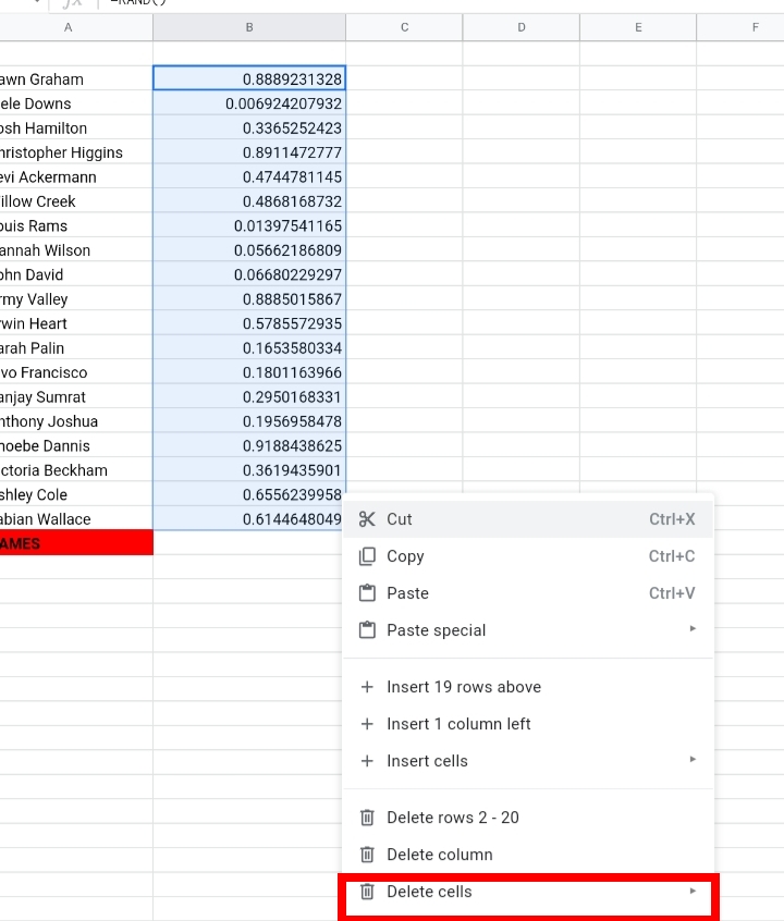
You might ask why we deleted the random numbers. This is because the RAND function is versatile and for every refresh or change made to the worksheet, the list shuffles automatically. Therefore, we prevent this from happening by deleting the RAND formula in column B.
Step 7: The list of names in column A is now shuffled at random.
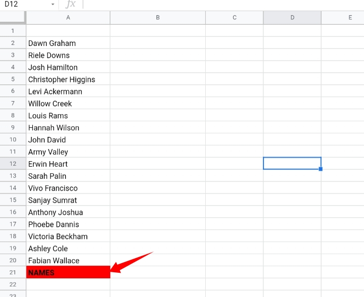
Note that The header of column A might be shuffled along with the other names because there was no specific range stated and the sort function examines the entire range of the worksheet. To correct this simply add a row above the first row, copy the header text and paste it back to the top cell.
The setback to this method is that due to the entire range being sorted if extra data is inputted into the same worksheet, the values would be affected as well but there’s another workaround for this method to ensure that only the selected range gets randomized.
Step 1: In the blank cell B2, input the Formula =RAND(). Press Enter on the keyboard.
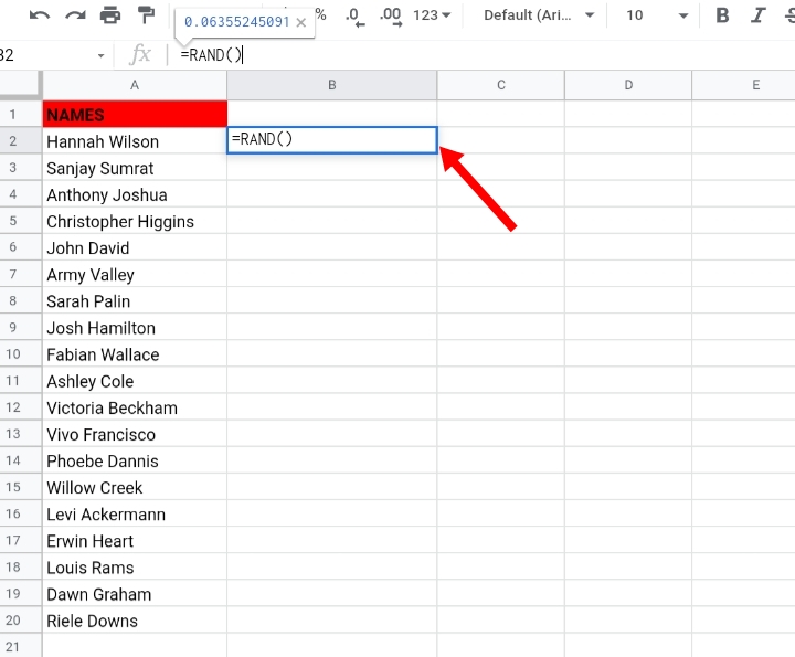
Step 2: As seen below, a random number in decimals is generated for the name in cell B2.
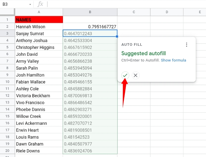
Step 3: Use the fill cube to copy and paste the formula into the remaining cells or by using the suggested autofill to automatically paste the random numbers for other cells in column B.
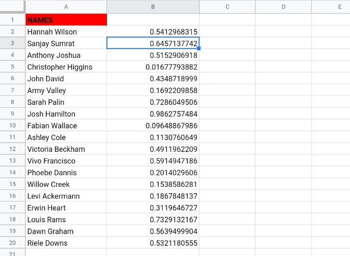
Step 4: Highlight the cell range of names along with the newly generated random numbers.
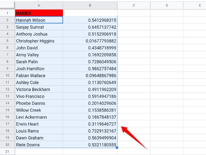
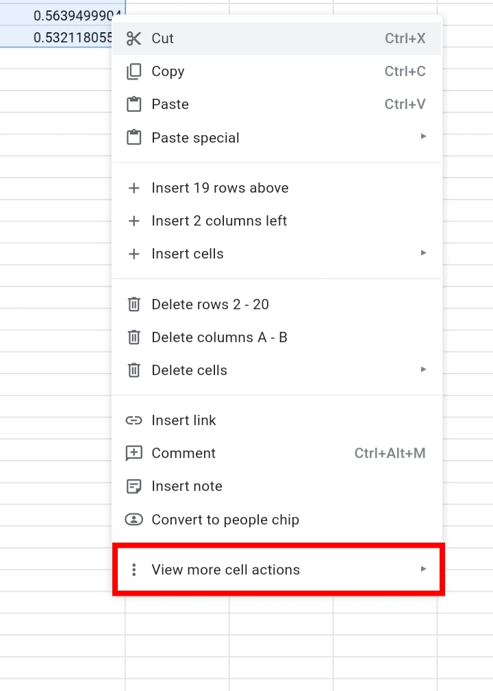
Step 5: Right-click on the selected cell range. From the drop-down menu, select View more cell actions, then select Sort Range.
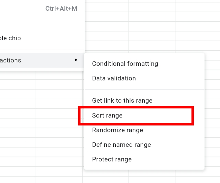
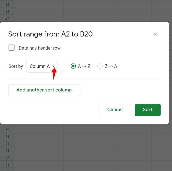
Step 6: The Sort Range tab is opened and displayed on the worksheet.
Step 7: Click on the drop-down arrow next to Sort by and select Column A.
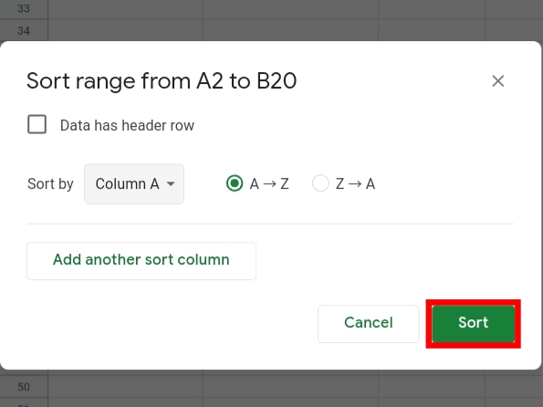
Step 8: Click on Sort.
Step 9: Highlight column B which comprises the random numbers and press the Ctrl key + Delete or Ctrl key + Backspace on the keyboard to delete the column content.
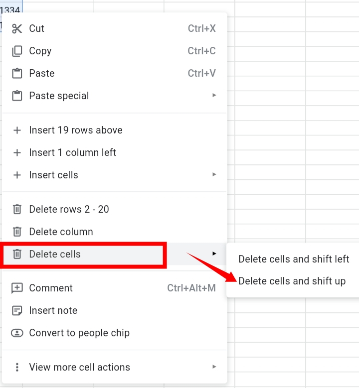
Step 10: Now, the selected column only gets randomized rather than the entire worksheet.
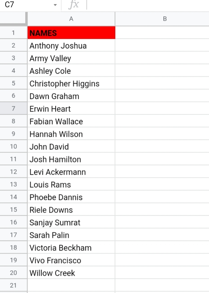
Method Three: How To Randomize a List in Google Sheets using a Formula.
This method is rather straightforward and quick to operate. This provides the same results as the previously discussed methods. The formula takes the syntax below.
=SORT(cell range, ARRAYFORMULA(RANDBETWEEN( SIGN( ROW( cell range)), 1000000)), True)
Substitute cell range in the formula as the range of the list. In the sample formula, the cell range is A2:A20.
Step 1: Input the formula into the column where you want the results displayed.
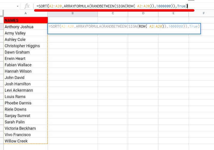
Step 2: Press Enter. The range of cells is automatically randomized.
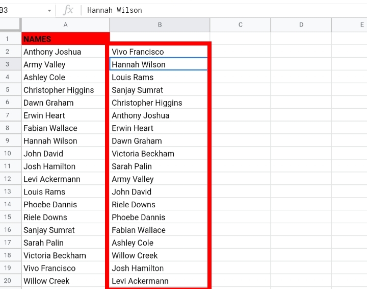
This method is very suitable for pairing two names together, as it doesn’t affect the names in the first column.
How To Select a Random Name from a List in Google Sheets.
In the previous sections, we have only discussed how to randomize a group of texts but what if you want to pick a random name or more than one random name.
The OFFSET function does the trick. The OFFSET function references a range of cells that are shifted or removed from a cell reference. The function takes the syntax below.
=OFFSET(cell_reference, offset_rows, offset_columns, [height], [width])
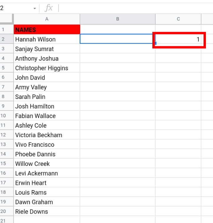
Step 1: In a random cell, for example, cell C2, enter the number of names that you want randomly picked. Since I want one name, I typed 1 in cell D5.
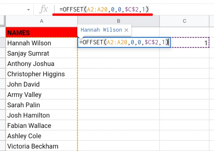
Step 2: Input the formula, =OFFSET(A2:A20, 0, 0, $C$2, 1)
Where A2:A20 represents the cell range.
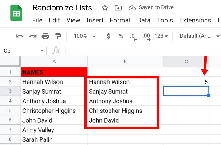
Step 3: Click Enter. A random name is picked out of the nineteen names in column A. If the number is changed in cell C2, the formula selects the names according to the number.
Final Thoughts.
This feature is really helpful as it gives the user control and flexibility of the content in the worksheet. Here, we have completely explained how to use the randomize feature properly. I hope you found this catalog helpful. Thanks for reading.


