Values that appear frequently in a worksheet are considered unique values. When working on large sets of data, you may want to extract these unique values across the columns of the selected worksheet.
In this tutorial, we are going to learn How To Create A Unique List Of Data Across Multiple Columns In Google Sheets.
What is the UNIQUE function?
Before we get into this topic, let’s understand what the UNIQUE function is and how it works. The UNIQUE function is a function that locates and extracts unique values while discarding
duplicate data. As said earlier, this function is most suitable when working with large datasets so that any replicated data is located and extracted from the worksheet. The UNIQUE function takes the syntax below.
=UNIQUE(cell range)
Where;
- Cell range- this is the range of data containing the unique values you want to be extracted.
How To Use the UNIQUE Function on One Column?
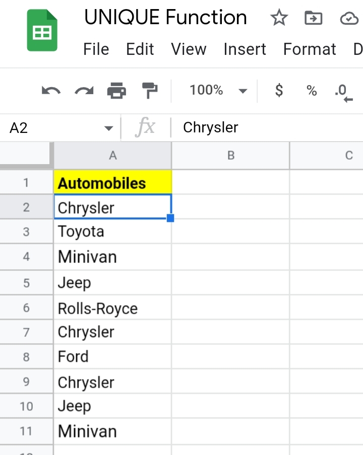
This is done by using a single column range as the cell range in the formula. By doing so, the unique values in the column are returned to the result cell. For example, the column below has examples of automobiles in column A.
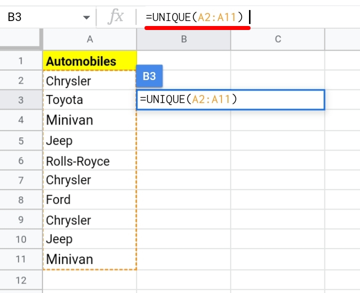
So in the result cell, we type in the formula, =UNIQUE(A2:A11)
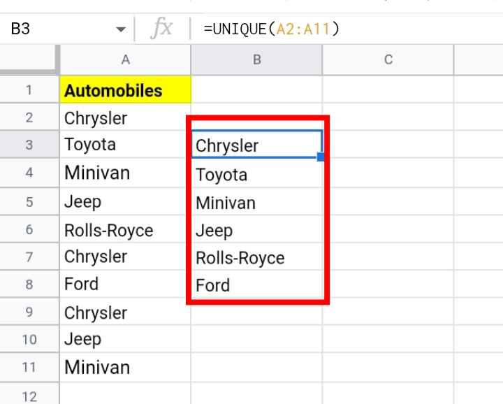
The unique values are located and extracted into the cells in column B.
How To Use the UNIQUE Function on Multiple Columns.
In case you want to extract unique values in multiple columns, you can use the UNIQUE function by simply adjusting the cell range to accommodate the extra columns.
Assuming you have to extract unique values from the multiple columns in the worksheet with the names of cars and their model brands in columns A and B respectively. The formula, =UNIQUE(A2:B11) is inputted in the result cell.
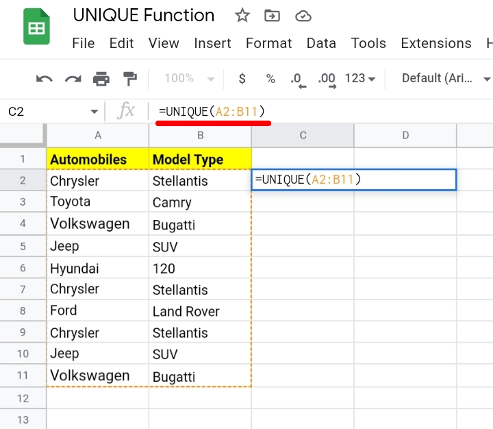
Each unique value returned for each column is displayed in columns C and D.
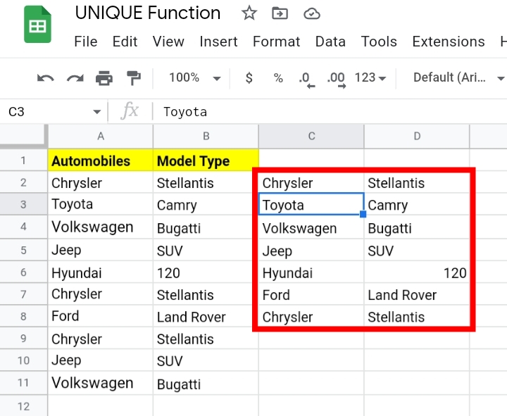
Using the UNIQUE function Across Multiple Columns.
The result above in the previous section will return unique functions from the selected cell range only but if you want to use UNIQUE functions across Multiple Columns, it would be done by
using the FLATTEN function. This function extracts the unique values across the multiple columns and places them in a single column. The combination formula of UNIQUE and FLATTEN would take the syntax below.
=UNIQUE(FLATTEN(cell range1,[cell range2,…])
Where;
- The cell range1 is the range containing the data from which you want to extract the duplicate values.
- Cell range2 is an optional parameter. Additional ranges are added here.
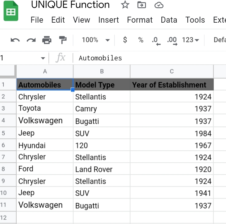
So in the sample worksheet used earlier, we have added a new column for the year of establishment of each automobile company. We are going to practice this using the worksheet.
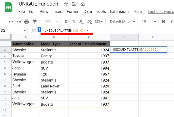
Select a result cell and input the formula =UNIQUE(FLATTEN(A2:C11))
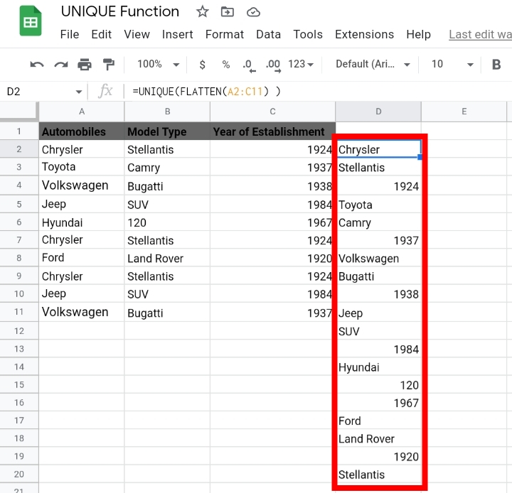
Click Enter and the unique or duplicate values are removed so that only one sample of each value is left in a single column.
Final Thoughts.
The UNIQUE function is very essential for returning values in Google Sheets. There are also alternative methods of extracting and removing duplicate values like the concatenate function.
Now you know How To Create A Unique List Of Data Across Multiple Columns In Google Sheets. Be sure to learn and understand this function properly and it’s sure to help out in your data entry projects. Thanks for reading.


