When the Checkbox feature was added to Google sheets in 2018, it was mainly used to tick out information from to-do lists, schedules and timetables.
It was discovered recently that checkboxes can also work in conjunction with conditional formatting in Google Sheets.
The conditional formatting applies color, conditions and formulas to the worksheet, making dissemination and evaluation of data easy.
In this tutorial, we are going to learn how to change the color of checkboxes when they are toggled.
How to Change the Checkbox color while Toggling in Google Sheets.
This is done in two ways.
- Conditional formatting formula to change checkbox colors.
- Conditional formatting to highlight the row ticked.
Method 1: Conditional formatting formula to change checkbox colors
This is a method that only changes the color of the checkbox without highlighting the whole row. In the sample worksheet below, we have a daily routine and the schedule of each chore.
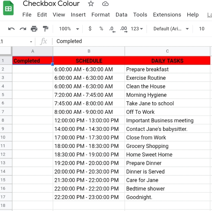
We are going to insert checkboxes into the worksheet and add color to them so that when a routine is completed it gets highlighted in the selected color.
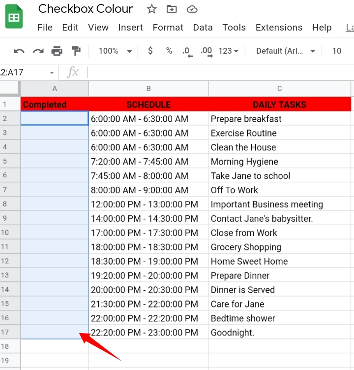
Step 1: Select a cell or range of cells where the checkboxes would be inserted.
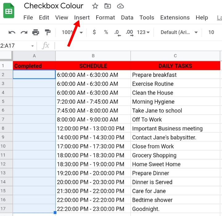
Step 2: Select Insert on the toolbar.
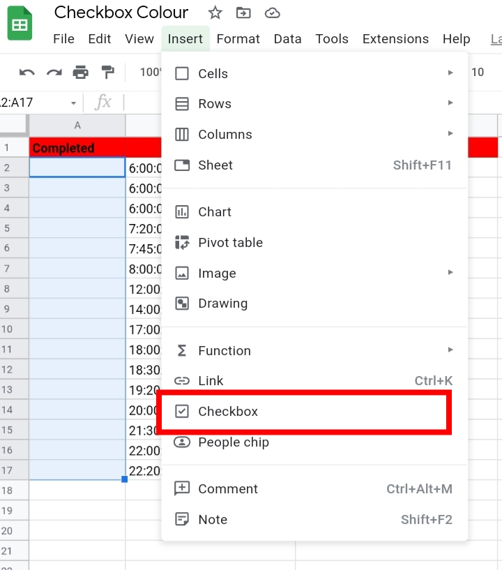
Step 3: From the drop-down menu displayed, select Checkbox.
Step 4: The checkboxes are inserted into the selected cells. The checkboxes can be ticked on or off the worksheet.
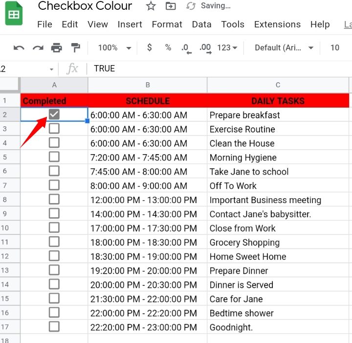
Now, we want to change the color of the checkboxes.
Step 5: Click on Format on the toolbar.

Step 6: From the menu, select Conditional Formatting.
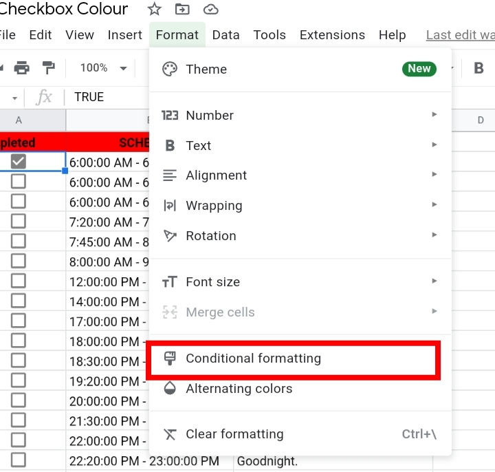
Step 7: The conditional formatting tab is opened on the right side of the worksheet.
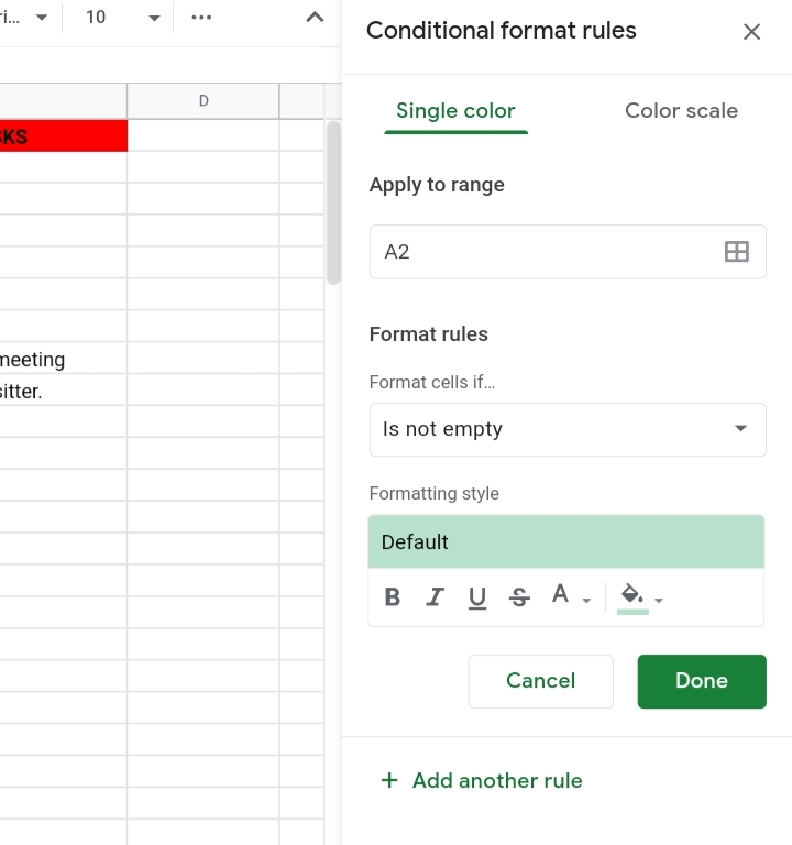
Step 8: Input the range of the checkboxes in the worksheet, that is A2:A17.
Step 9: Under Format rules, select Is equal to.
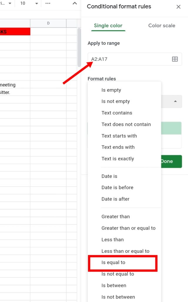
Step 10: Enter the condition as TRUE. This means that when the box is checked, it is true it becomes colored while if it gets unchecked, it is false and the color is removed.
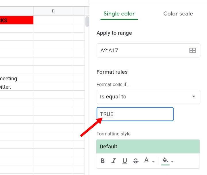
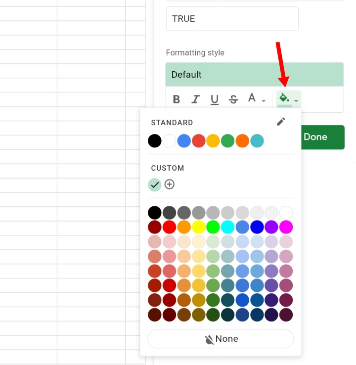
Step 11: Click on the fill color icon here and select any color of your choice.
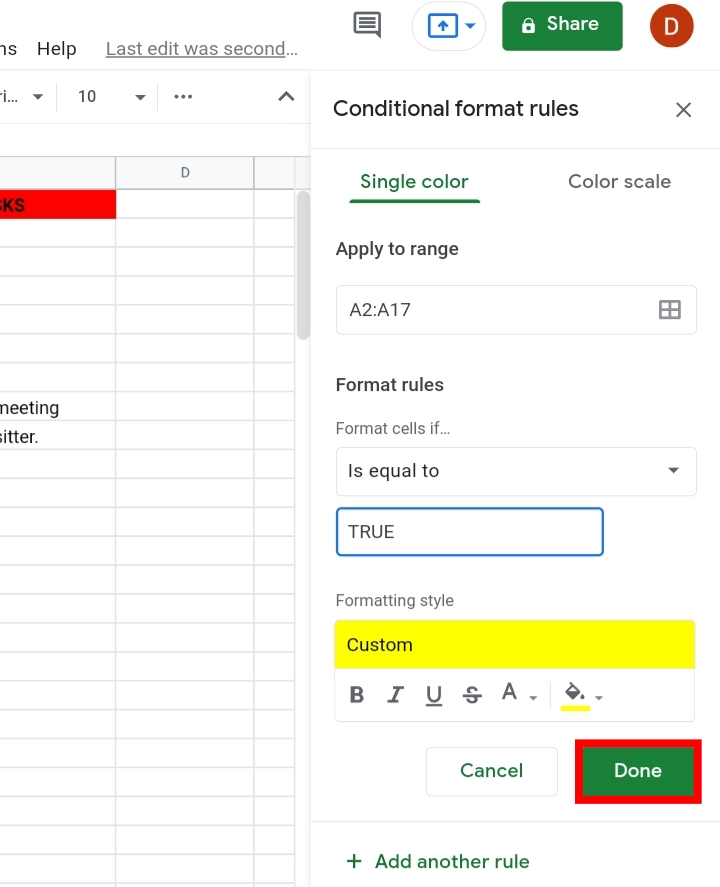
Step 12: Click Done.
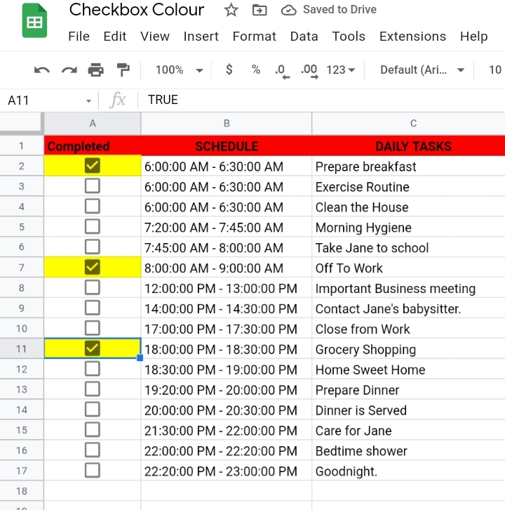
If a checkbox is selected, it becomes colored and if it’s unchecked, the color is removed.
Method 2: Conditional formatting to highlight the row ticked.
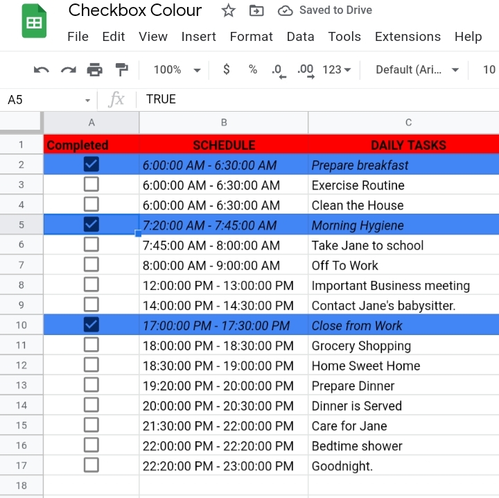
This is the second method used to color checkboxes, but the entire row is also highlighted when the checkbox is checked.
Step 1: Click on Format on the toolbar.
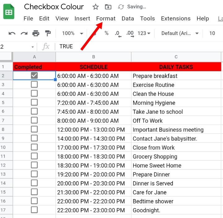
Step 2: From the menu, select Conditional Formatting.

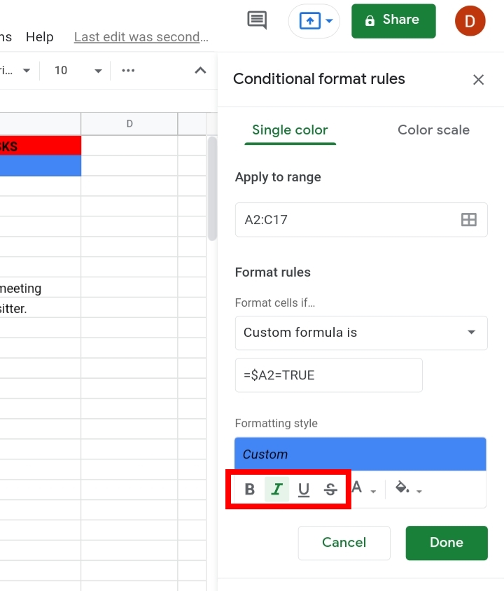
Step 3: The conditional formatting tab is opened on the right side of the worksheet. Input the entire range of the worksheet.
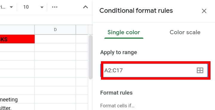
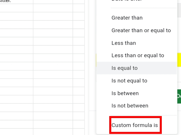
Step 4: Click on the drop-down arrow to Format rules, and select the Custom Formula Is.
Step 5: Input the formula as =$A2=TRUE
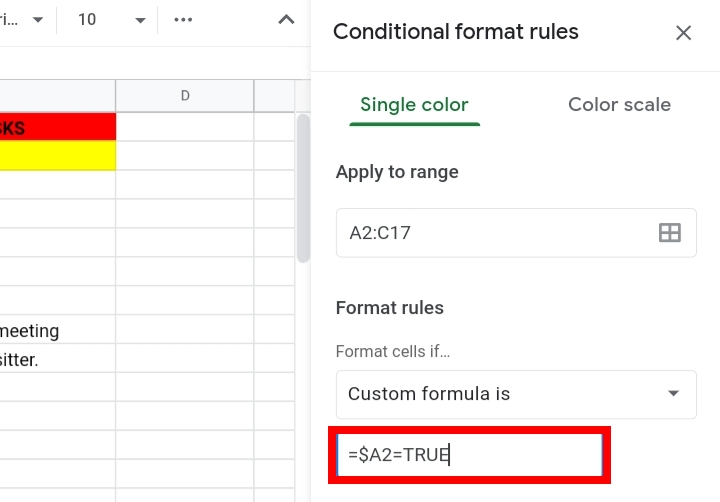
Step 6: Under formatting style, click on the fill color icon and select any color. You can also add extra formats like Bold, Italics or Strikethroughs so that when the checkbox is ticked, the respective texts are also highlighted and formatted to the selected style.
The Logic behind the Checkbox color Changes.
The reason for the color changes in the checkbox is that an unchecked box is FALSE by default. When checked, the value changes to TRUE.
It is an important factor that aids the color formatting of the checkbox. To prove this, select a cell with a single checkbox and input the formula =A1 into another empty cell.
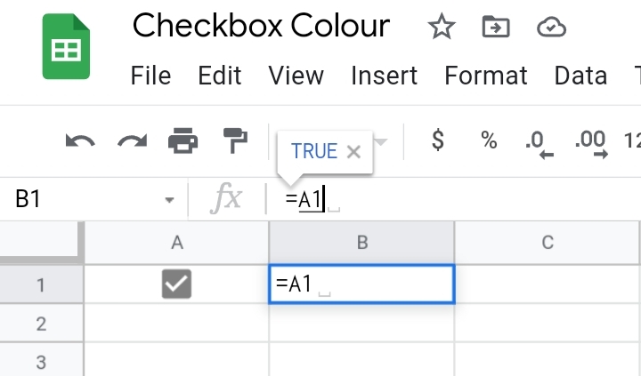
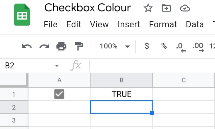
This would return the default values of the cell to TRUE and if it becomes unchecked, it changes to FALSE.
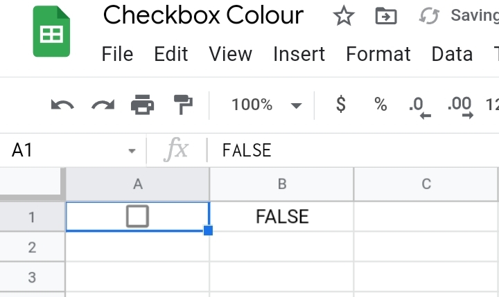
Note that the default values of the checkbox can also be changed through Data validation.
Click on Data, then Data validation.
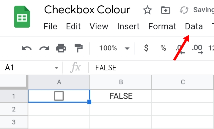
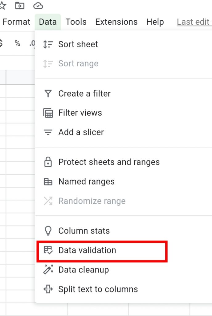
Click on the cell range textbox and select the cell or range of cells with the checkboxes.
Under the criteria tab, select the Checkbox.
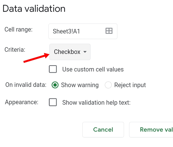
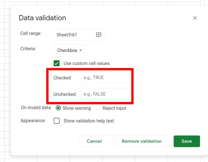
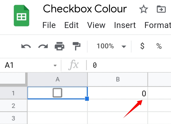
Click on Use Custom cell values. The two default values are TRUE and FALSE. Let’s change it to 1 and 0.
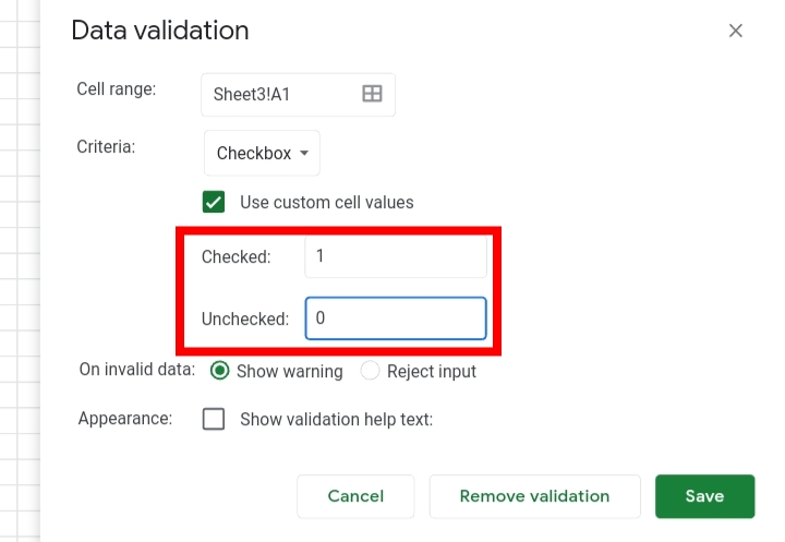
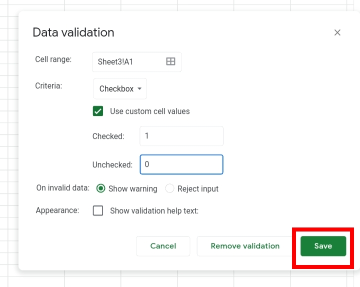
Click Save.
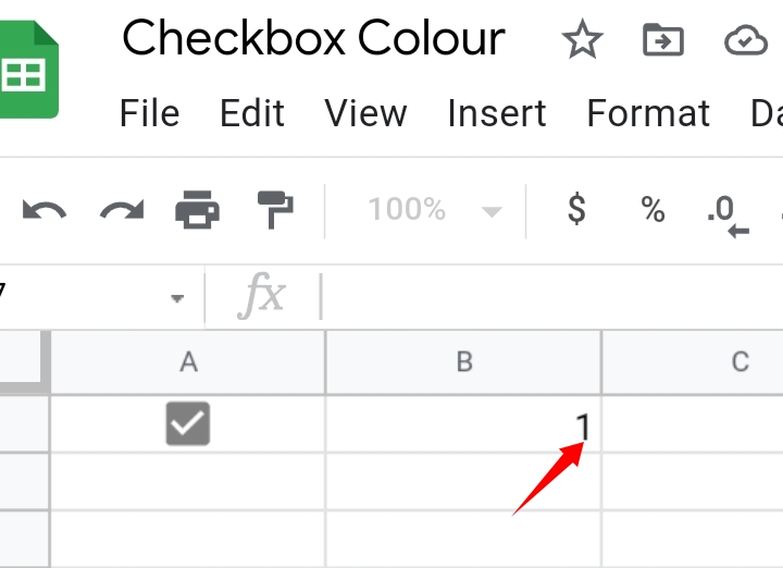
By typing the formula =A2 into an empty cell. When checked, the returned value is 1 while when unchecked, the returned value is 0.
Final Thoughts
Now, you know how to Change the Checkbox Color While Toggling in Google Sheets in 2022 using two different methods.
Checkboxes are very efficient features especially when applied with conditional formatting. I hope you found this article helpful. Thanks for reading.


