Drop-down lists are features used to provide a specific range of options to a user. It aids an accurate track of data and reduces the chances of errors and misspellings. Drop-down lists are also important components of dashboards, dynamic charts, and monitoring projects.
These significant tools can also be created with Google sheets. In this tutorial, we are going to learn more about dropdown lists and how they are added to a worksheet.
How To Add Yes/No Drop Down Lists in Google Sheets
In the sample data below, we have a questionnaire handed out to a group of high school students about basic scientific facts and knowledge.
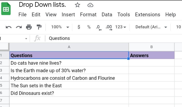
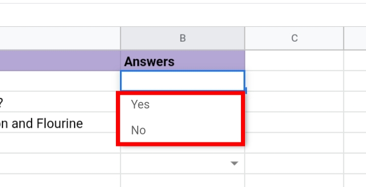
Each student is required to give a Yes or No response to each question stated by selecting their answers from the drop-down lists. This is where we create a Yes or No drop-down list from which they can select by following the steps below.
Step 1: Select the cells in column B which is where the drop-down list appears.
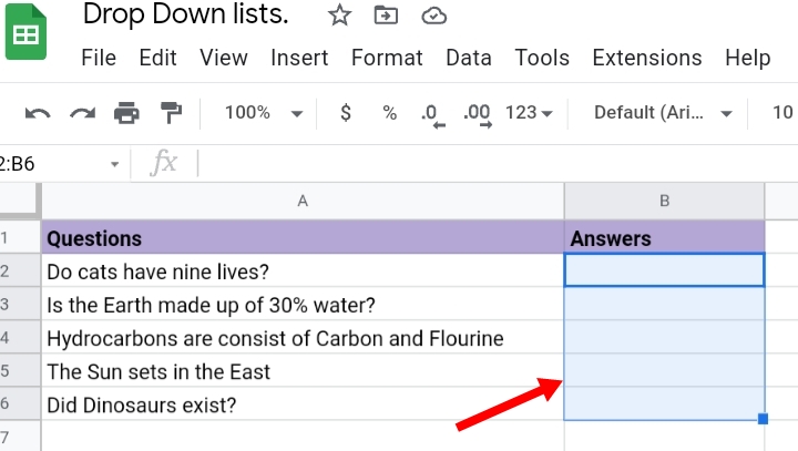
Step 2: Right-click on the selected cells. A drop-down menu is produced, scroll down and select View more cell actions.
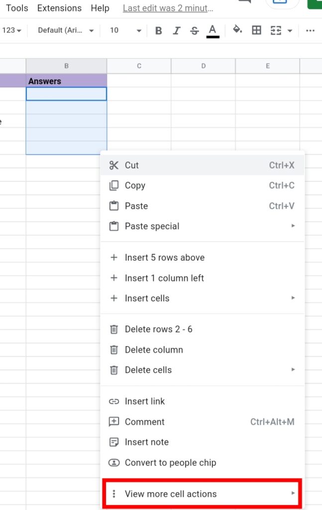
Then, select Data Validation.

Alternatively, you can go to Data on the toolbar.
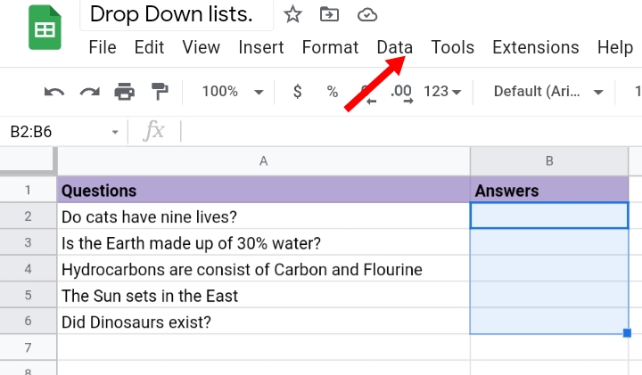
Under the drop-down menu, select Data Validation. Data validation helps to distinguish the options entered in the drop-down list.

Step 3: A pop up is shown on the worksheet. Although the cell range is automatically inputted into the textbox, properly inspect and ensure the sheet name and cell ranges are correctly inputted.
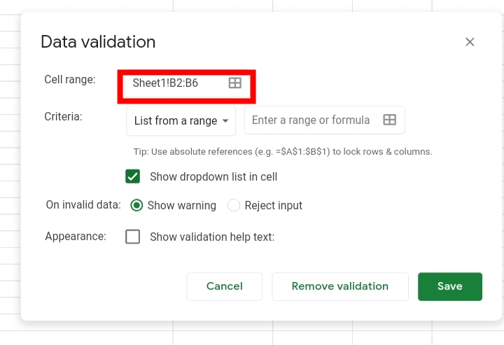
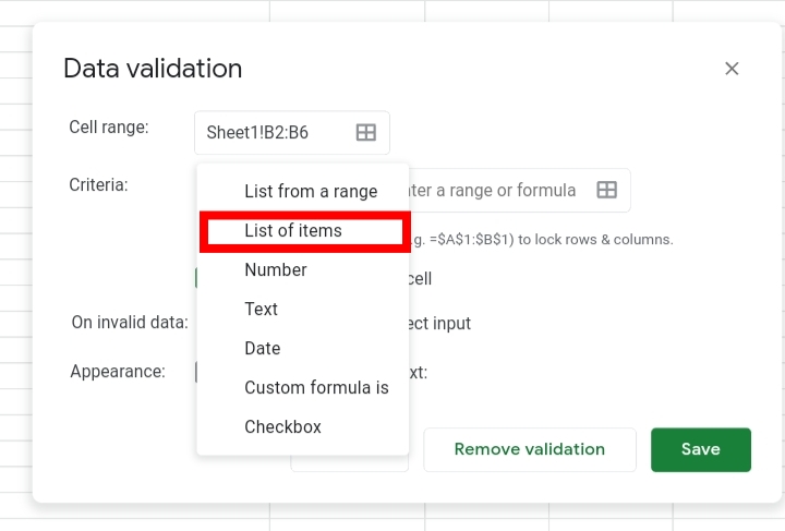
Under the criteria category, click on the drop-down arrow and select List of Items.
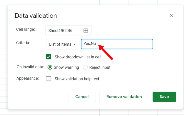
Step 4: Input Yes, No into the textbox provided.
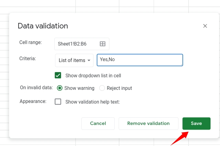
Step 5: Click Save.
Step 6: Several dropdown arrows are placed into the selected cells.
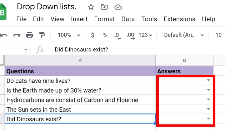
If you click on them, a Yes or No drop-down list is displayed there.
Also, if you created only one drop-down list for one cell, you can spread the validation to other cells by copying the cell and pasting it.
Step 1: Select the cell with the new drop-down list.
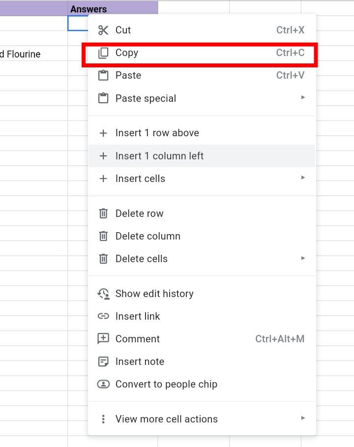
Step 2: Right-click on the cell. From the drop-down menu, select Copy or press the keyboard shortcut, Control key + C. The borderline of the cell changes to short blue broken lines. This signifies the cell’s content has been copied successfully.
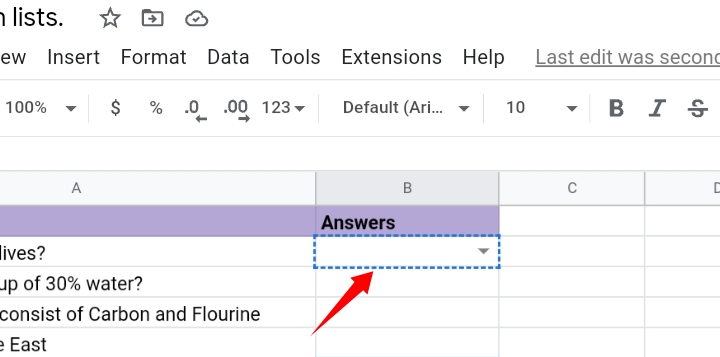
Step 3: Highlight the other cells which you want the validation pasted.
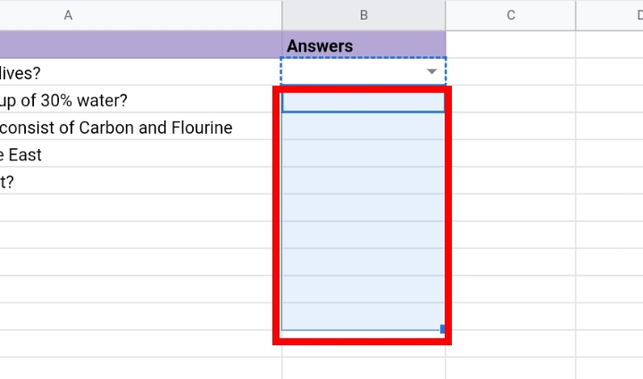
Step 4: Right-click on the highlighted cells. From the dropdown menu, select Paste Special.
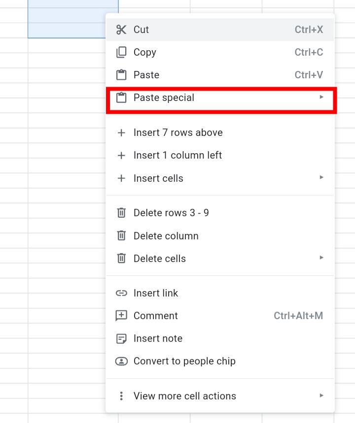
Step 5: From the options available, select Paste Data Validation Only.
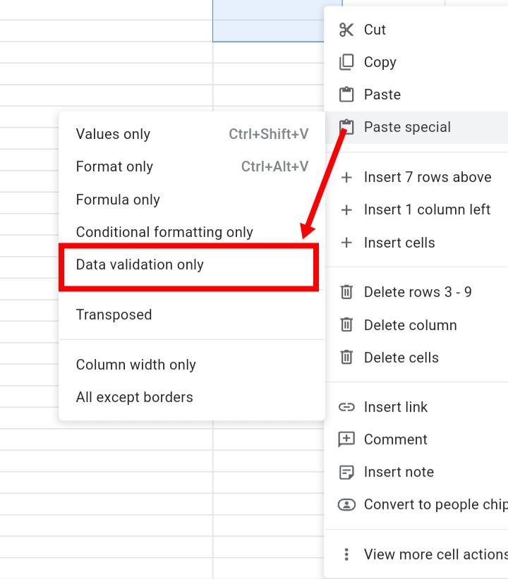
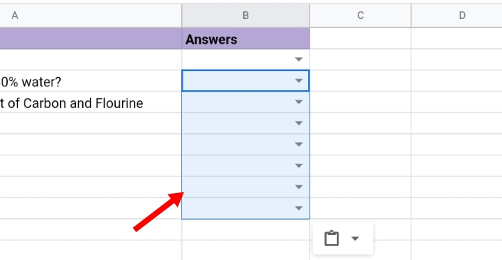
Step 6: More drop-down lists are pasted into other cells in the worksheet.
How To Add More than Yes or No in the Drop-down list in Google Sheets
For instance, some students were indecisive about the questions asked and couldn’t choose between yes or no. Well, you can add extra options to the drop-down list by following the phases stated below.
Step 1: Select the cells in column B with the drop-down arrows.
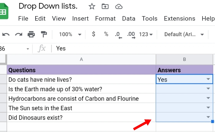
Step 2: Right-click on the selected cells. A drop-down menu is produced, click on more cell actions.

Select Data Validation.
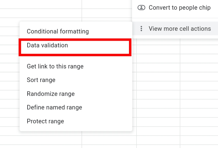
Also, you can go to Data on the toolbar.

From the drop-down menu, select Data Validation.

Step 3: In the textbox with Yes, No, let’s add “Maybe” into the options. It is typed together with a comma separating each word.
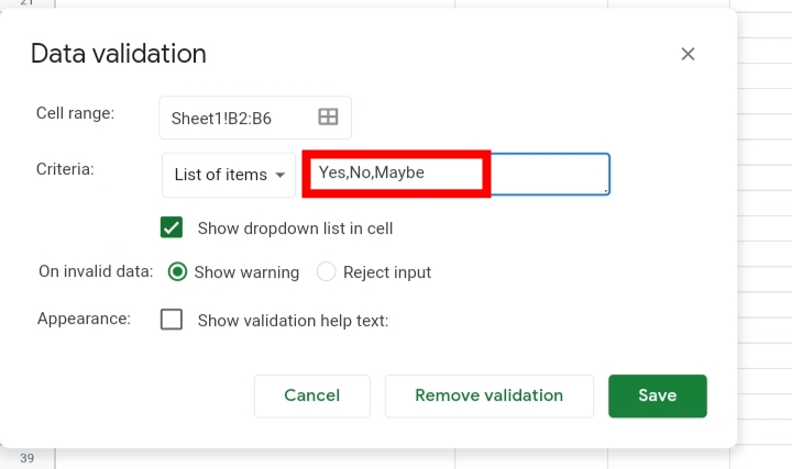
Step 4: Click Save.
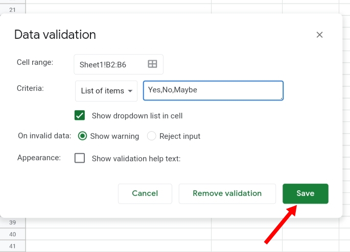
Step 5: By clicking on the drop-down arrow, the options are displayed there, with the Maybe option included. So students with uncertain answers can select the Maybe option from the list.
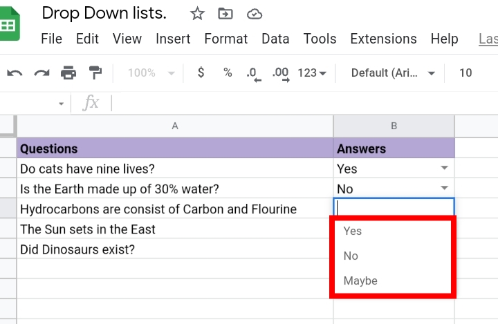
This proves that dropdown lists in Google Sheets are extremely flexible and can be edited however you want it.
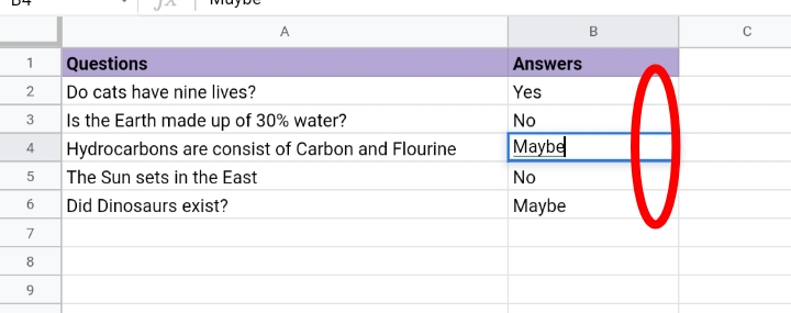
Note that if another random text is inputted into a dropdown cell, a tiny red triangle appears on the top right corner of the cell, this means the text is an error and shouldn’t be placed there.
How to Remove a Drop-down list in Google Sheets
Removing dropdown lists is very easy to execute by repeating the steps taken to create the drop-down list.
Step 1: Select the cells in column B with the drop-down lists.
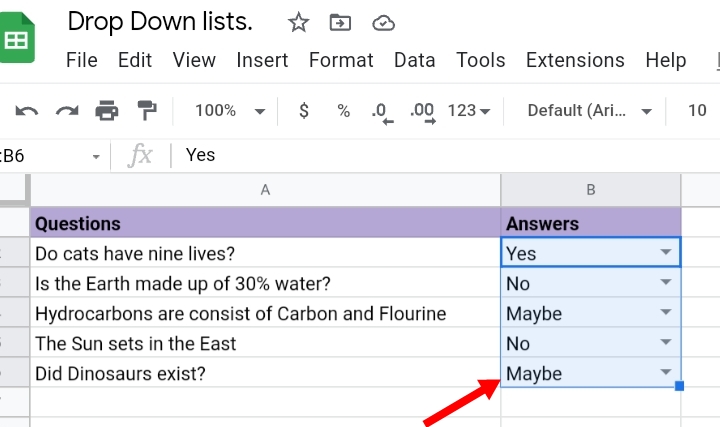
Step 2: Right-click on the selected cells. A drop-down menu is produced, scroll down and select Data Validation.
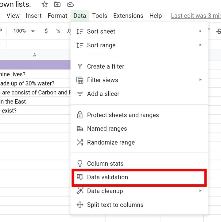
Alternatively, you can go to Data on the toolbar.

From the drop-down menu, select Data Validation.
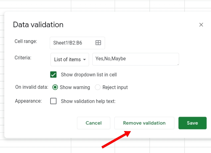
Step 3: From the displayed pop-up, click on Remove Validation.
The drop-down lists are now removed and the texts become ordinary as they can be edited by normal means.
Closing Thoughts
Drop-down lists are great tools for keeping track of data. When used in combination with the VLOOKUP and FILTER functions, they serve as dynamic search engines that can extract data based on a particular setting and can also create dynamic charts in Google Sheets.
With this tutorial, creating and operating drop-down lists have been made effortless. I hope you found this guide enlightening and useful. Thanks for reading.


