Diagonal lines are tools used to separate headers representing different columns from each other. Unlike Microsoft Excel, there isn’t an inbuilt feature for creating diagonal lines in Google sheets. Therefore, we are going to improvise on a few ways to insert diagonal lines in cells.
There are three known methods used to insert diagonals in cells and each method would be explained in detail to improve understanding.
The sample worksheet below does not have headers to indicate the dataset in column A to column M. We would insert diagonals in A1 to separate the headers of each data set.
Method 1: Insert a Diagonal line Using the Tilt feature.
This feature is employed when you want to divide your cell into two parts. For instance, if a cell contains two headers or titles and you want to separate them to represent their respective columns, the tilt feature is used.
Step 1: Select the row you want to dissect.
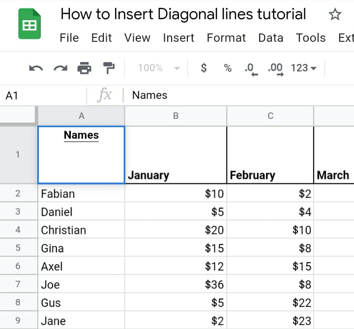
Step 2: Press the Alt + Enter simultaneously on your keyboard. This causes a line break between the two headers.
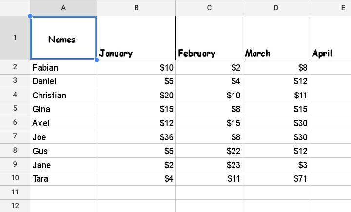
Step 3: Type in multiple dash lines.
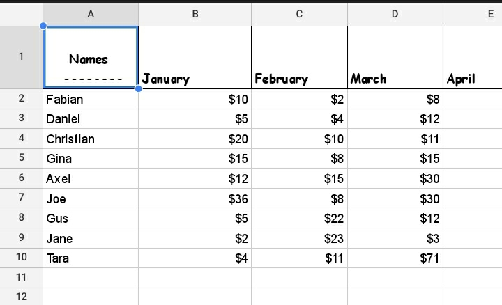
Step 4: Press Alt + Enter again on the keyboard to cause another line break.
Step 5: Type the second title below the dash lines.
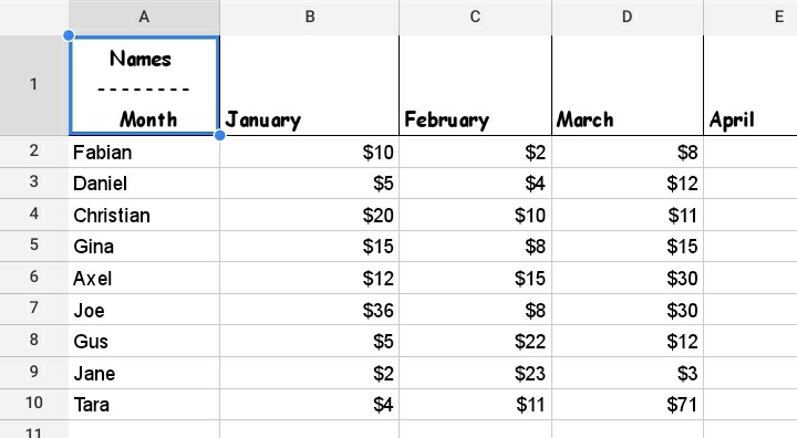
Step 6: Select cell A1.
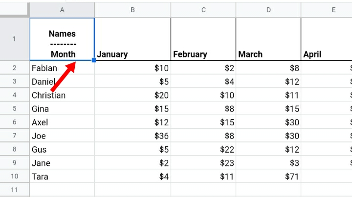
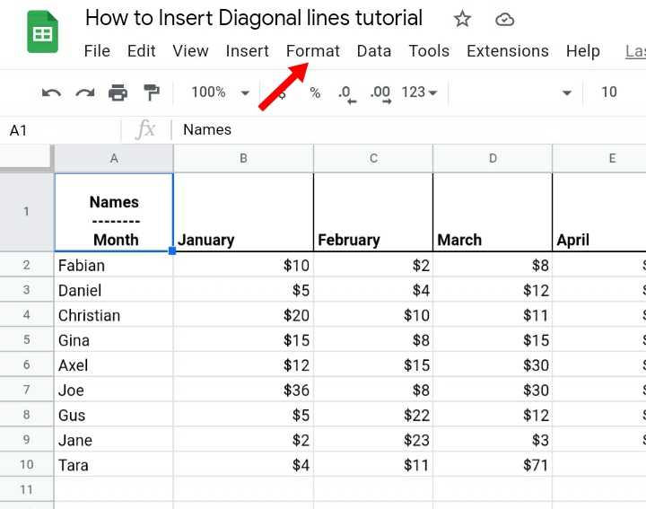
Step 7: Click on Format on the toolbar.
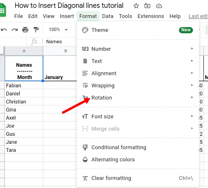
Step 8: Click on Rotation.
Step 9: You can click on either the tilt up or tilt down option, depending on the direction you want your diagonal to face.
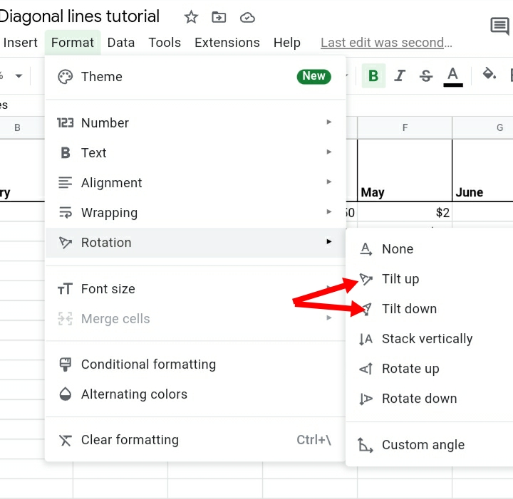
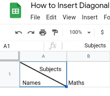
Step 10: Click on tilt-up and it produces the results as seen below.
Alternatively:
You have to follow previous 6 step then start 7 from here
Step 7: Click on the three dots arranged horizontally on the toolbar.
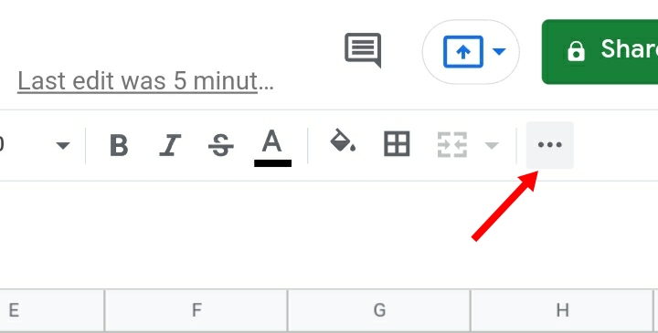
Step 8: You can click on the cell rotation icon on the toolbar.
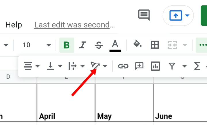
Step 9: You can select the tilt up or tilt down option or click on the degree icon to select the angle of tilt and direction you want your diagonal line and headers to face.
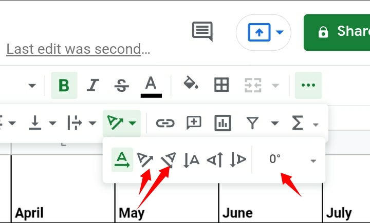
If you click on the degree icon, it displays a list of degrees with negative and positive values.
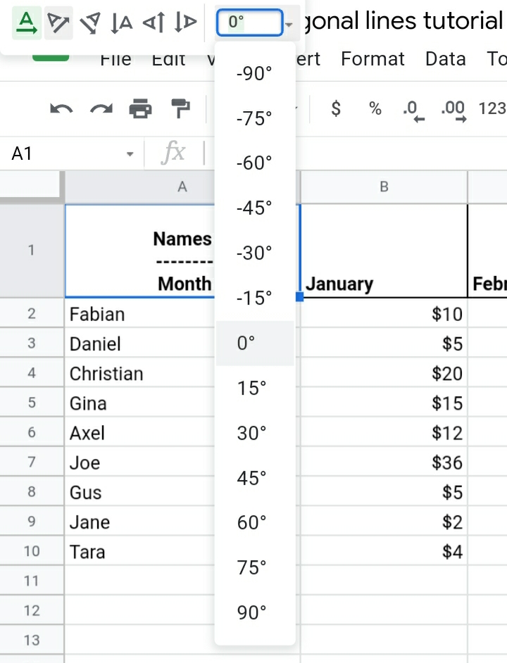
Method 2: Drawing a Diagonal line and Add the text.
Although this technique has a few disadvantages, the drawing method is particularly easy to learn and understand with the following steps below.
Step 1: Click on Insert.
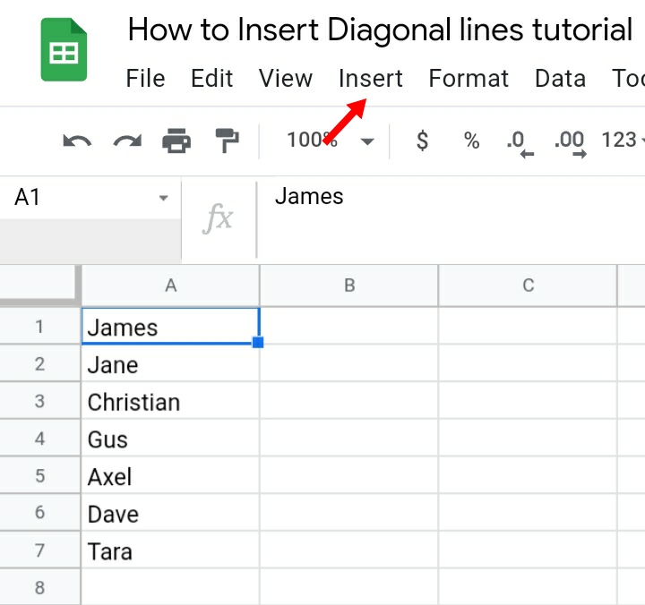
Step 2: Select Drawing.
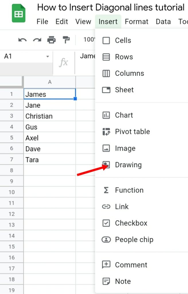
Step 3: Click on the drop-down arrow.
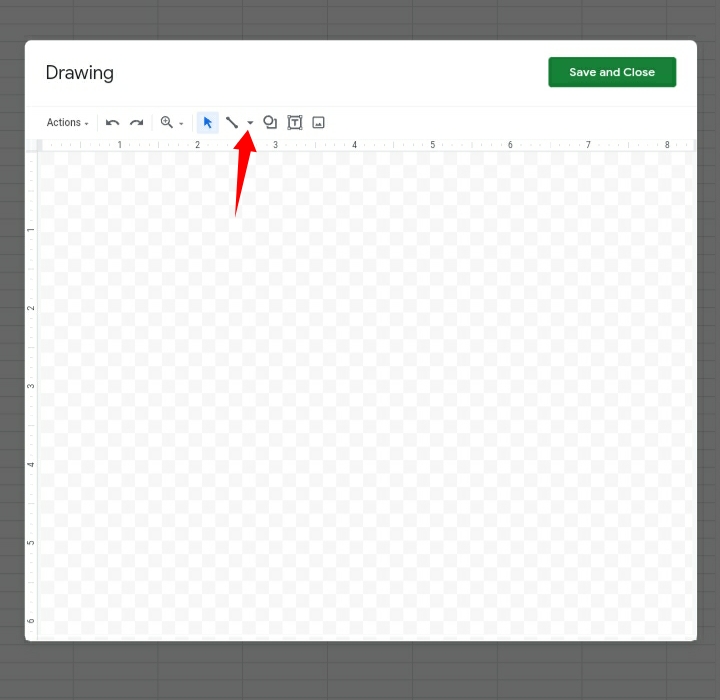
Step 4: Select the Line option here.
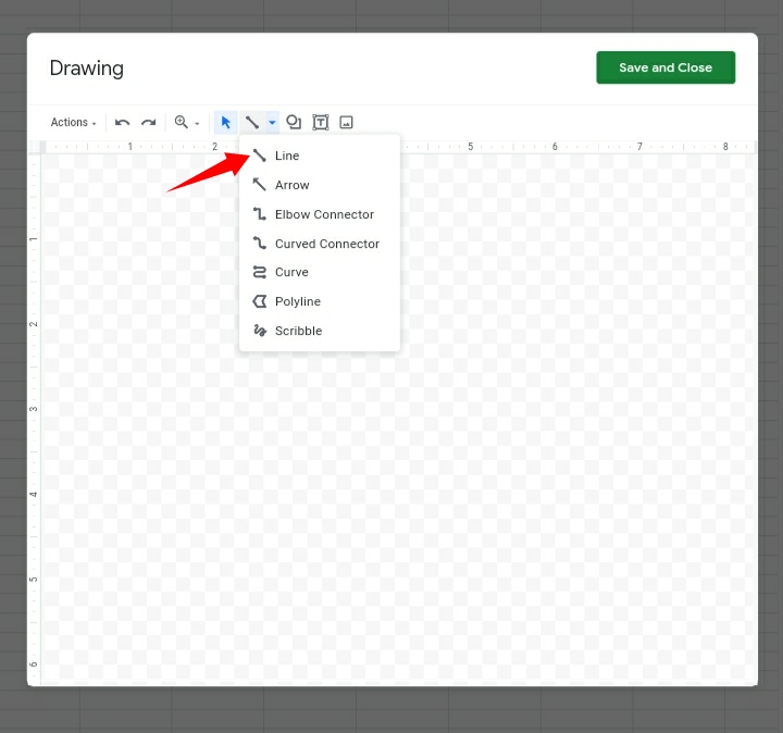
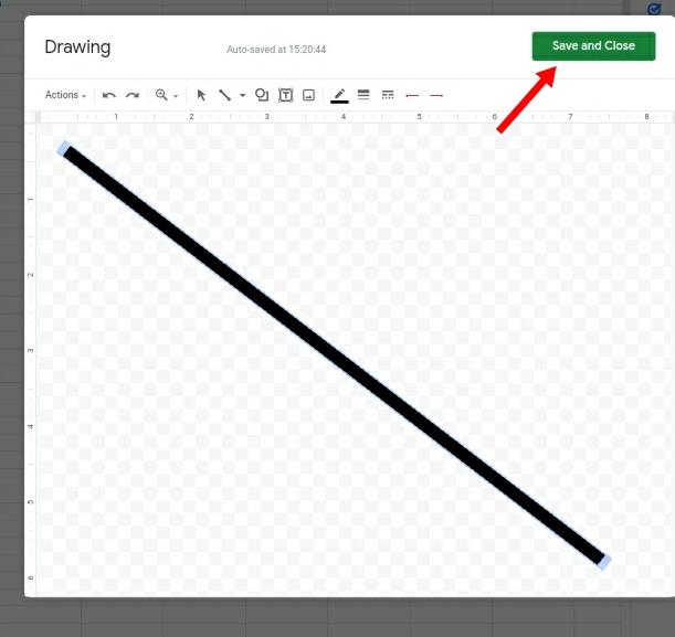
Step 5: A page is shown on the sheet. Draw a diagonal line across the sheet.
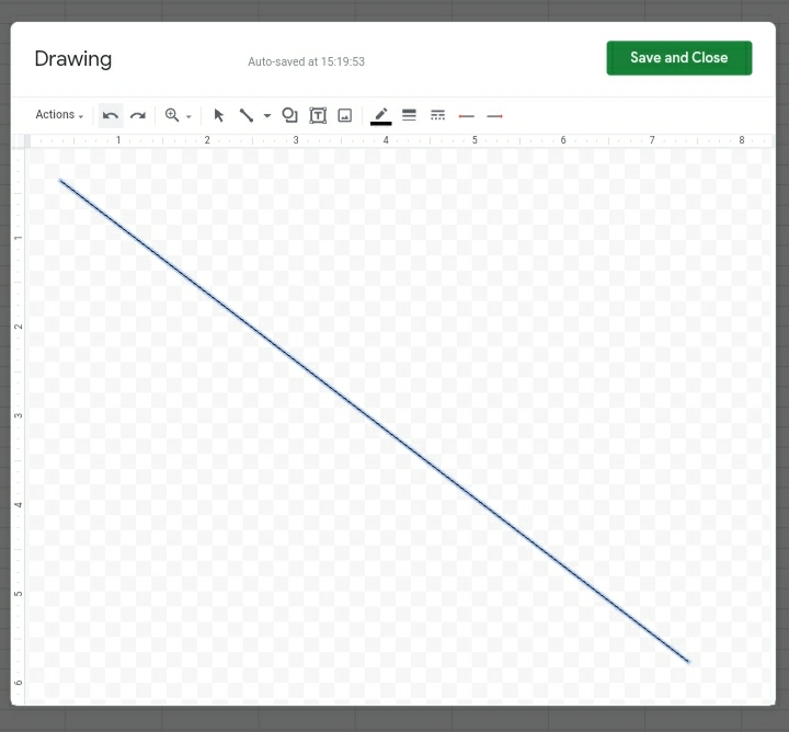
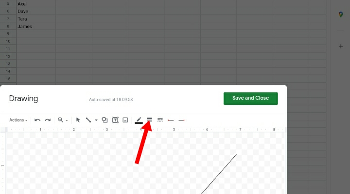
Step 6: Click on the Line Weight icon.
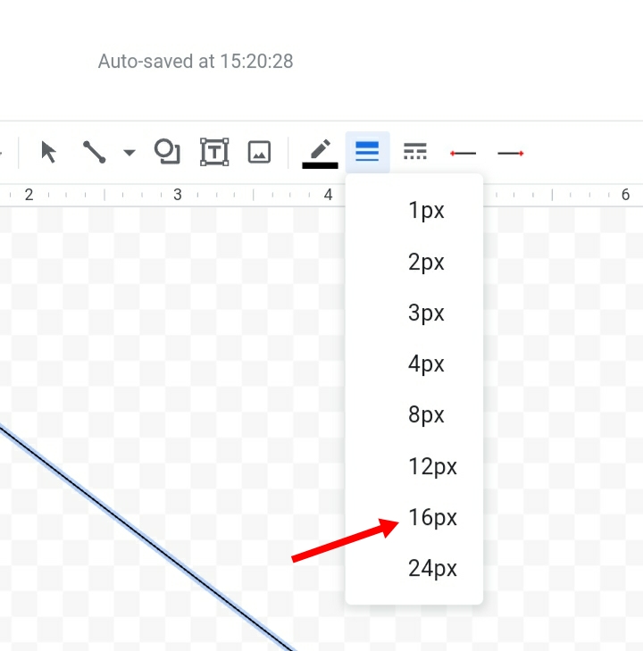
Step 7: Increase the line weight to about 16px to improve the thickness and visibility of the line.
Step 8: Click on Save and Close.
Step 9: Press Enter on the keyboard and the line would appear on the worksheet.
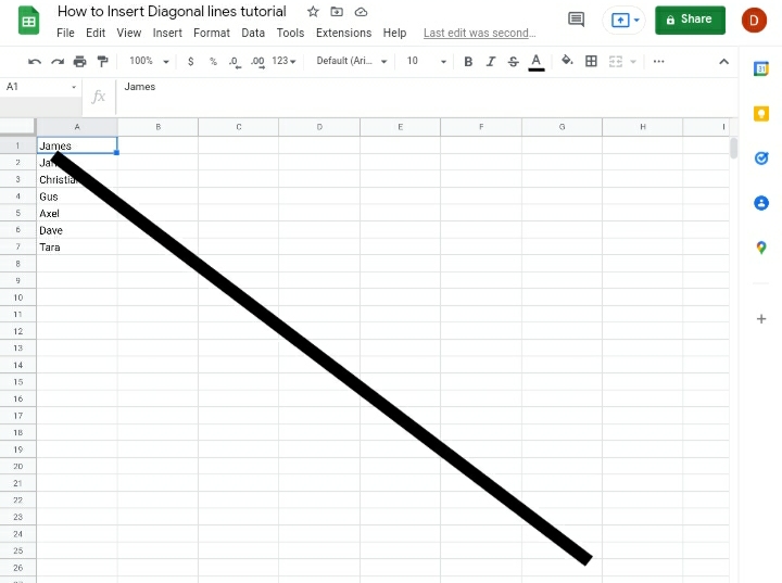
Step 10: Using the mouse, click on the sides of the diagonal and drag it in. The diagonal line size is decreased to fit into the cell.
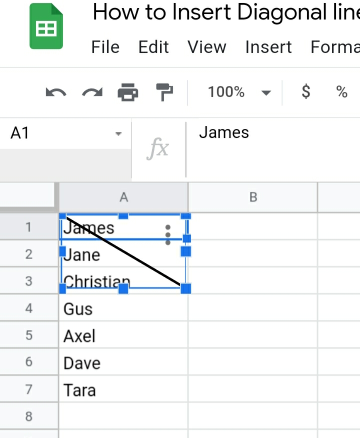
Step 11: Adjust the diagonal line to fit properly into the row.
Step 12: Type in the respective headers in the cell above and below the diagonal line to indicate the columns.
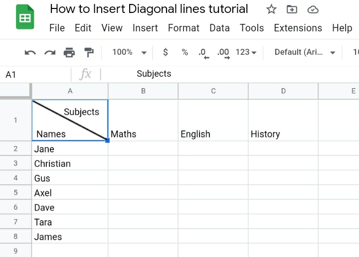
You can also create another diagonal with this method in case you want to make an X which can be used for the cancellation of data in a cell.
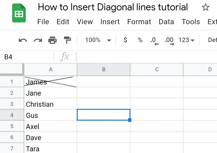
Note: This technique has a few disadvantages.
- The line is not placed in the cell but over the cell. It doesn’t become part of the cell component.
- When additional editing or tools are used on the sheet such as Zoom, it only affects the worksheet, leaving the diagonal line unaffected
Due to the disadvantages listed above, it is not considered the best method for inserting diagonal lines in cells but it does serve its purpose as a diagonal line and gives a better-looking result than the tilt method.
Method 3: Insertion of Diagonal lines in Blank Cell Using the Sparkline Function.
This method is specifically used when you want to insert a diagonal line in a blank cell. The sparkling function is used to create miniature charts in Google sheets. With the formula below, one can create a chart consisting of only one diagonal line.
=SPARKLINE({1,0},{“color”, “black”})
This formula would be used to put a diagonal line into the blank cell.
Step 1: Input the formula into the blank cell.
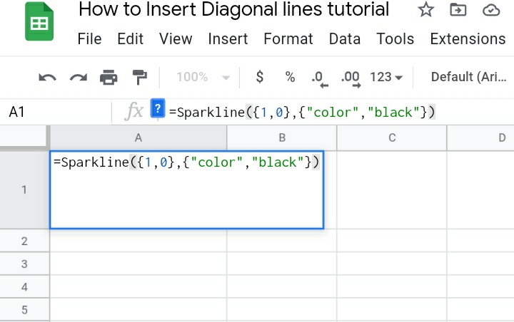
Step 2: Click Enter
Step 3: A diagonal line is displayed in cell A1 of your worksheet.
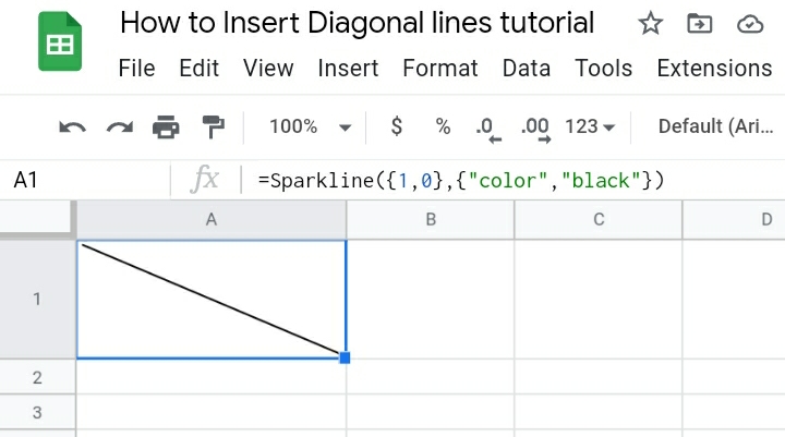
Note: You can also change the direction and color of the diagonal by swapping the 1, 0 to 0, 1 and changing the color ” black” to “yellow” or any color of choice in the formula. The formula looks like this:
=SPARKLINE({0,1}, {“color”, “yellow”})
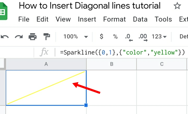
This method is considered the fastest and best method because the formula makes the diagonal line become a part of the cell, unlike the two previous methods which mean that whatever filter or edit is done on the cell, the diagonal line would be affected too.
Final Thoughts:
Although the diagonal line feature is temporarily absent in Google sheets, with the above steps and detailed explanation, this has been made easy for both beginners and intermediate google sheets users.
Put in the required effort and practice and you would become a master in all three methods. I hope you enjoyed this tutorial, thank you.


