As usual, Google sheets provides a wide range of actions and benefits, which includes inserting the current date and time in your worksheet.
Instead of inputting the time and date manually on your worksheet.
Google sheets have inbuilt functions and formulas that perform such tasks and update the time and date daily.
In this tutorial, we are going to discuss the three methods used to insert time and dates in Google sheets.
Adding the Current Date and time using the NOW function.
The NOW function is a volatile and dynamic function. It is easy to operate and requires no additional parameters in its formula syntax. This function inserts both the date and time. The default format of the inserted date is DD/MM/YY which is the standard format.
The NOW formula takes the syntax below.
=NOW()
As stated earlier, there are no required parameters. If values or cell references are inputted in the formula, it would result in an error.
Step 1: In an empty cell, type in the formula =NOW()
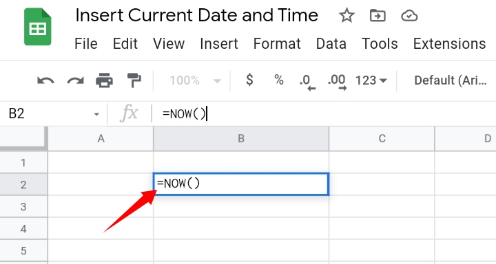
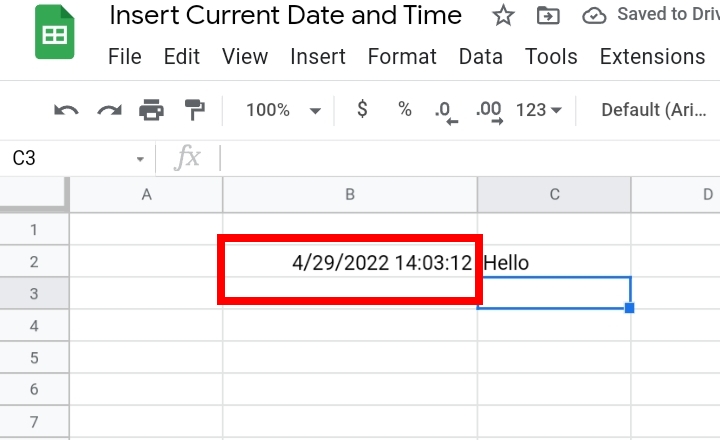
Step 2: Press Enter on the keyboard. The present date and time are inserted into the worksheet.
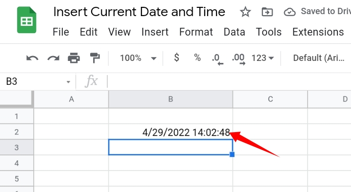
Also, due to time zones globally, you can change the format of the inserted data.
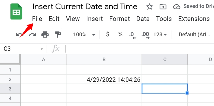
Step 1: Select File on the toolbar.
Step 2: Select Settings.
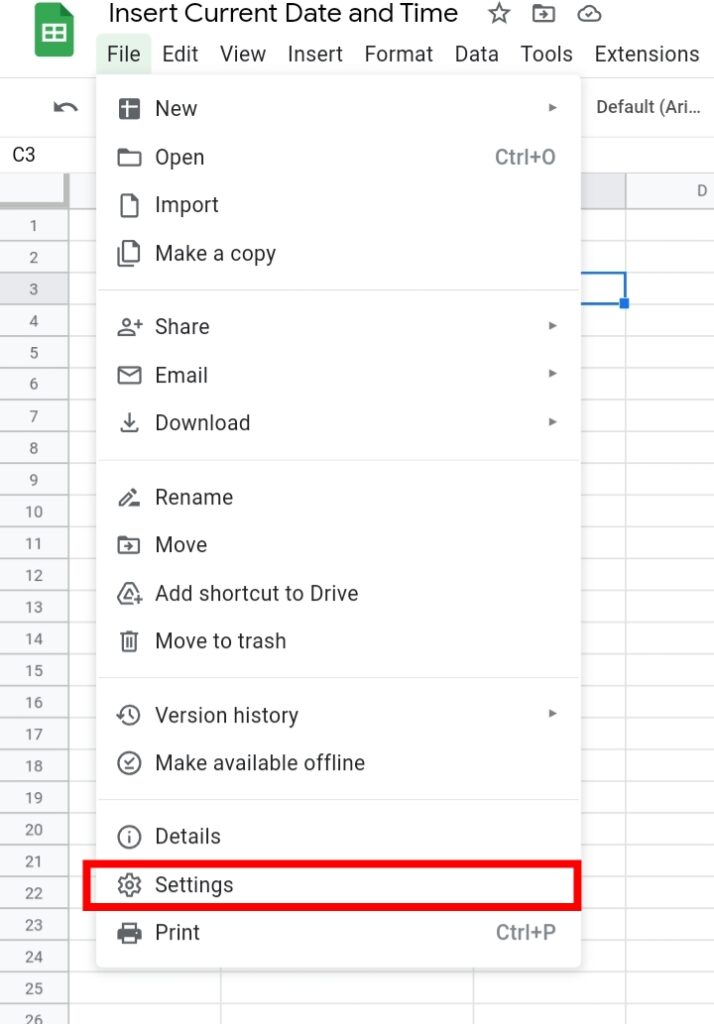
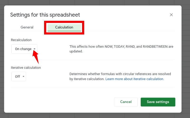
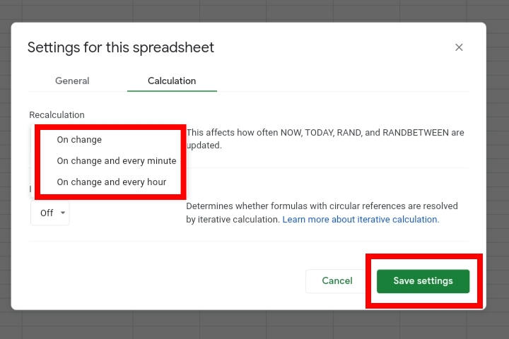
Step 3: Click on the Calculation tab. Select the Recalculation from the drop-down menu displayed.
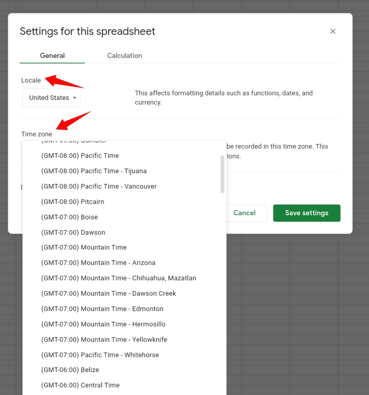
You can also select locale and time zones under the General tab.
This method is as easy as pie and it dynamically recalculates as time passes by, when any change or refresh is made on the worksheet.
Check out How To Add A Date Picker In Google Sheets.
Finding The Date and time Using the TODAY function.
This function is similar to the NOW function in terms of its versatility and dynamic nature but it only inserts the current date. The function takes the following syntax.
=TODAY()
The parentheses are required blank, if filled could result in an error.
This function also recalculates automatically as days pass by. Past days can be inserted by adding and subtracting the number of days and if it’s by a year past or a year further, you add or subtract by 365 days.
Step 1: In an empty cell, type in the formula =TODAY()
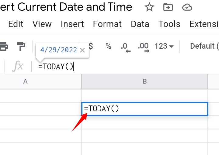
Step 2: Press Enter on the keyboard. The present date is inserted into the worksheet.
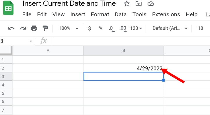
As said earlier, the default format is automatically placed on the inserted time, but it can be changed using the Format tool. This method also applies to the NOW function.
Step 1: Select the cell or range of cells containing the inserted time and date.
Step 2: Select Format on the toolbar.

Step 3: From the drop-down menu, select Number.

Step 4: Another list is displayed, select Date. To display the present time only, you’d select Time rather.
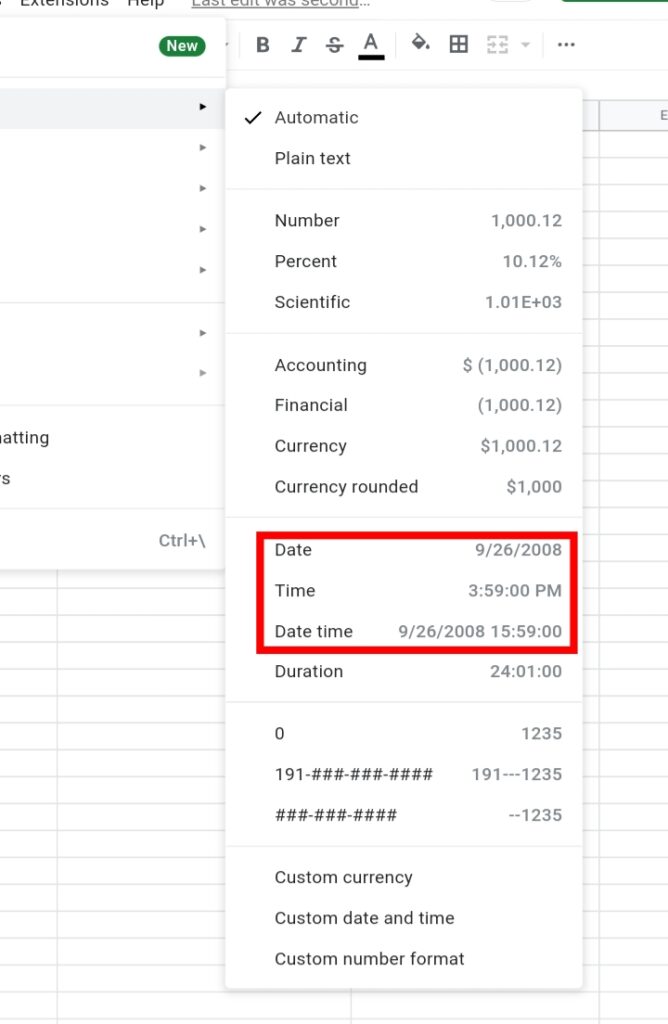
Also, you can customize the Date and Time format.
Step 1: Select the cell or range of cells containing the inserted time and date.
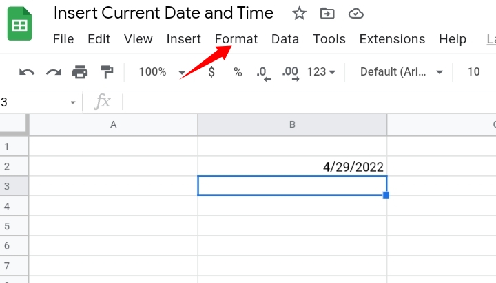
Step 2: Select Format on the toolbar.
Step 3: From the drop-down menu, select Number.
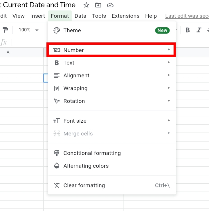
Step 4: Select Custom Date and Time. Additional formatting alternatives are also found here.
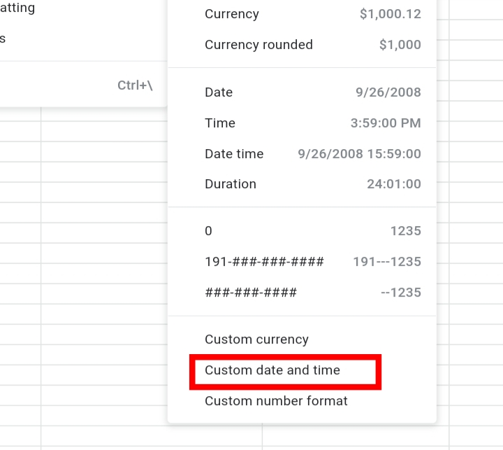
Now, you can format the text, date, time, numbers, and characters like the slash etcetera. You can select and apply a format.
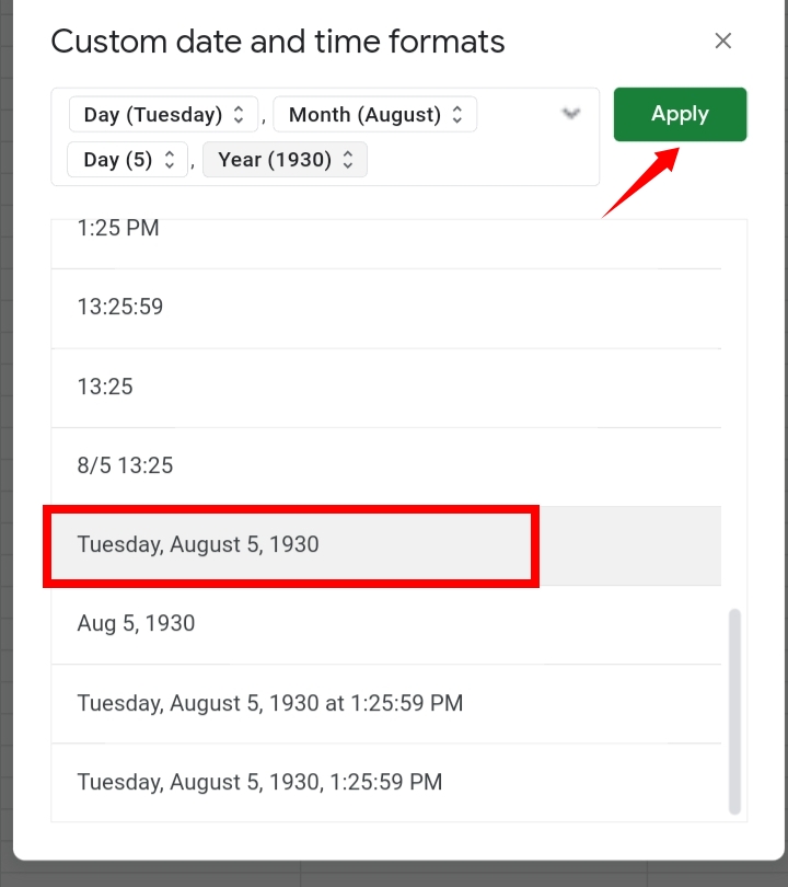
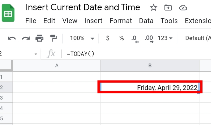
With the applied format, the TODAY and NOW functions are used to insert the current date and time in your worksheet.
Insert Static Dates into Google Sheets.
Suppose you don’t want the dates and times on the worksheet to change constantly, you can use the method to insert a static date and time into your Google Sheet. This technique is quite easy to understand and quick to use. It is done by using a keyboard function.
- To insert a static date in a cell, you use the keyboard shortcut, Ctrl key + ; (semicolon)
- To insert a static time into a cell, you use the keyboard shortcut, Ctrl key + Shift + : (colon)
Note that the dates and times are static and do not change as other modifications are made on the worksheet.
Final Thoughts.
Above, we covered this topic fully and successfully. The insert dates are very important especially when you are keeping track of specific items or keeping a sales record in your Google Sheet.
I hope you found this article informative and useful. Thanks for reading.


