Gridlines are lines that separate the cells and columns throughout the worksheet. They are seen around the cells in a worksheet. Sometimes, when working with data on the worksheet, you may want to seclude a part of the worksheet, by hiding other guidelines to emphasize the separated part of the data.
In this tutorial, we will discuss and learn how to remove, add and show gridlines in Google Sheets and also how to hide gridlines when you want to print the data.
How To Hide Gridlines in the Worksheet in Google Sheets.
Using the worksheet below, we want to hide the gridlines of some students’ grade reports.
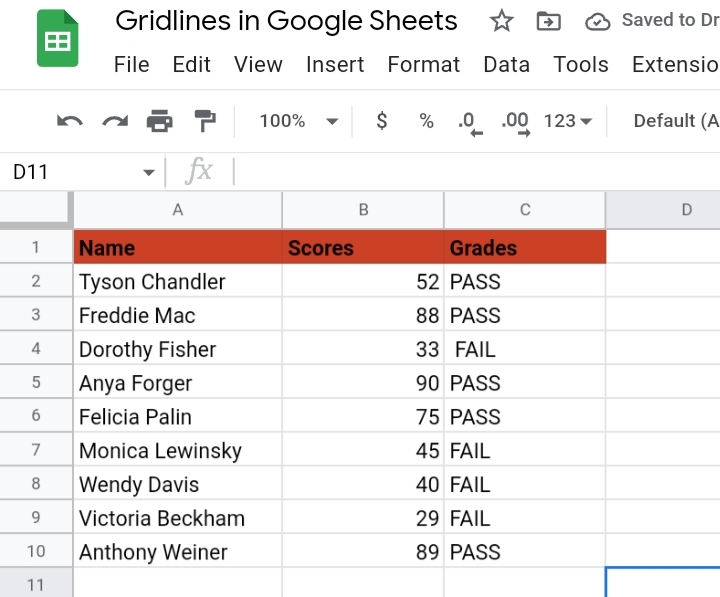
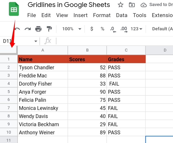
Step 1: Select the cell range of data you want to hide the gridlines. If you want to hide all gridlines in the entire sheet, click on the grey box on the top left corner of the worksheet.
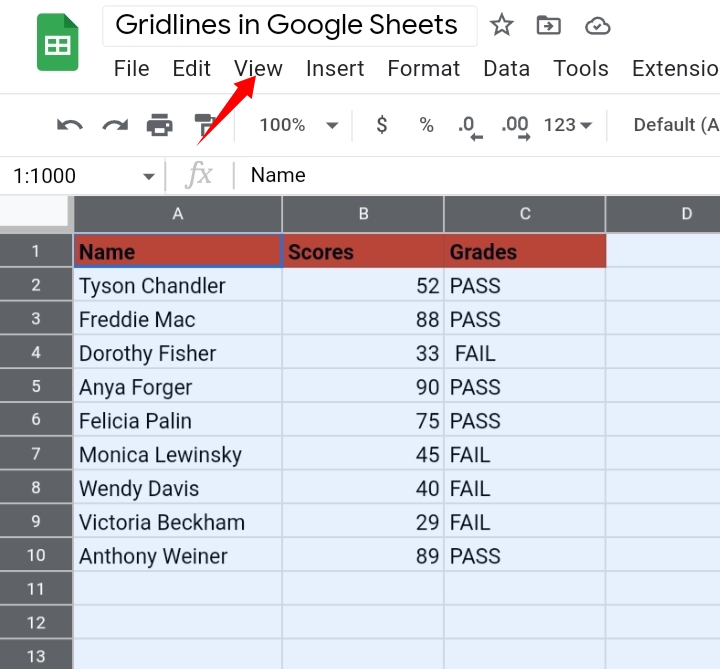
Step 2: Navigate to the toolbar and click on View.
Step 3: In the drop-down menu displayed, search and select Show.
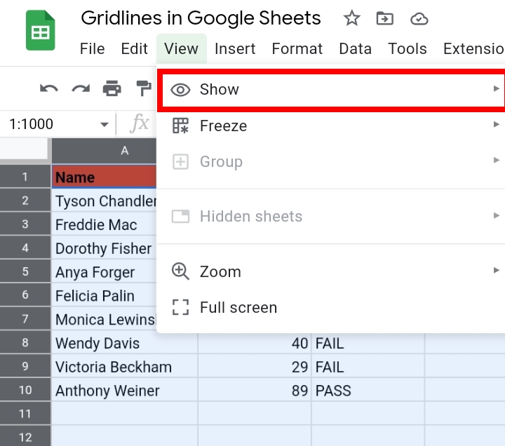
Step 4: Other options are displayed, select Gridlines.
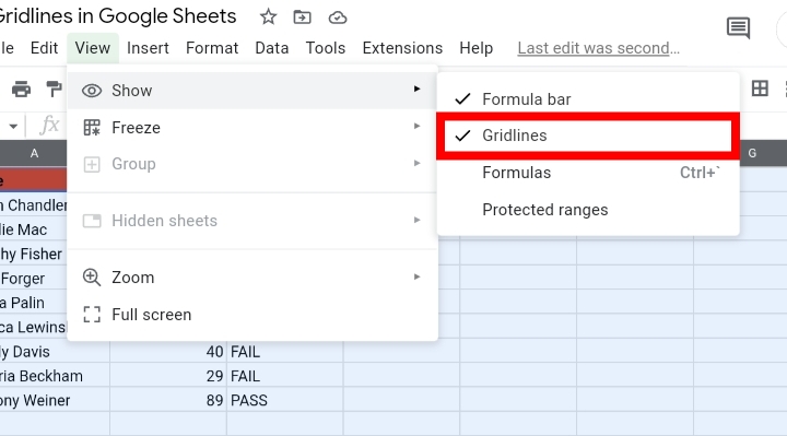
This would hide the gridlines of the selected cell range or the entire worksheet.
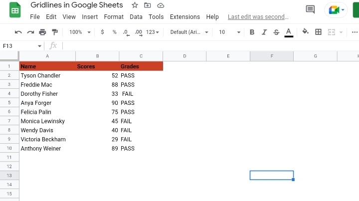
Note that this method acts as a toggle switch. If you want to add or show the gridlines, you follow the steps above too.
How To Hide Gridlines in Google Sheets when Printed.
In case you want to print out your worksheet with the gridlines and not have the grid lines printed in the final result, Google sheets has a way of achieving this and it is done in these quick and easy steps.
Step 1: Select the cell range or the entire worksheet you want to be printed.
Step 2: Navigate the File option on the toolbar.
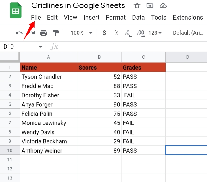
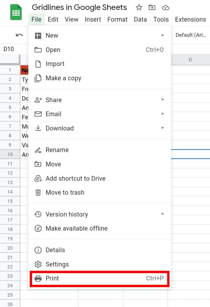
Step 3: From the drop-down menu displayed, search and select Print. Alternatively, you can use the shortcut key on the keyboard, Ctrl key + P.
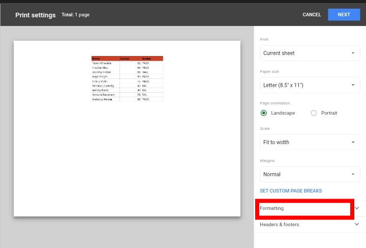
Step 4: The Print settings tab is opened. Click on the Formatting options.
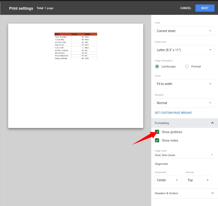
Step 5: Untick the “Show Gridlines“.
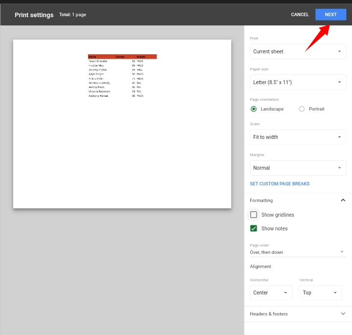
Step 6: Click on Next.
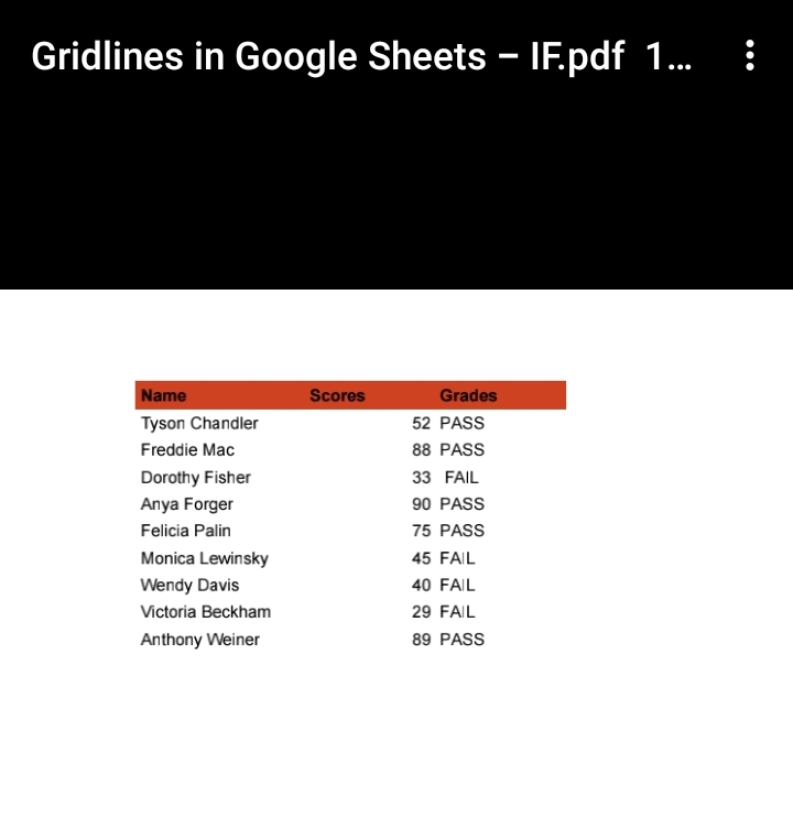
The printed worksheet has its gridlines hidden or removed.
How To Show Gridlines in Google Sheets.
For instance, you want to show some gridlines in a particular area in your worksheet and hide it in the remaining areas. It can be done in the following steps.
Step 1: Select the cell range of data you want to show the gridlines. If you want to show all gridlines in the entire sheet, click on the grey box on the top left corner of the worksheet.
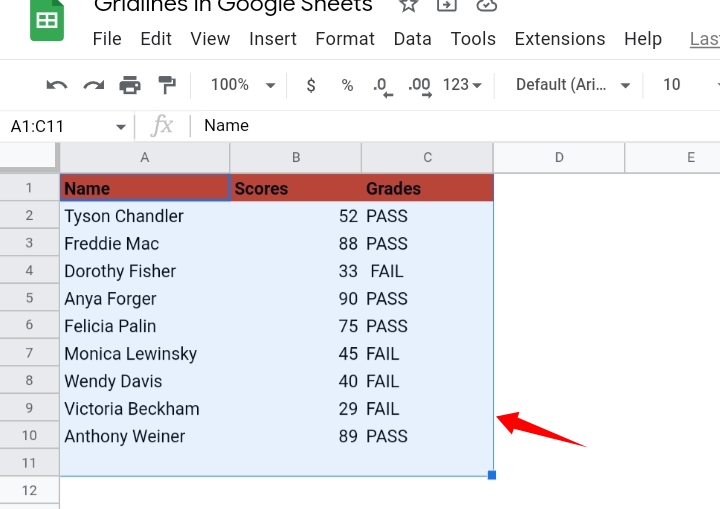
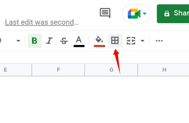
Step 2: Navigate to the toolbar and click on the Border Style icon.
Step 3: Select and apply the border of the cell range where you want the gridlines added.
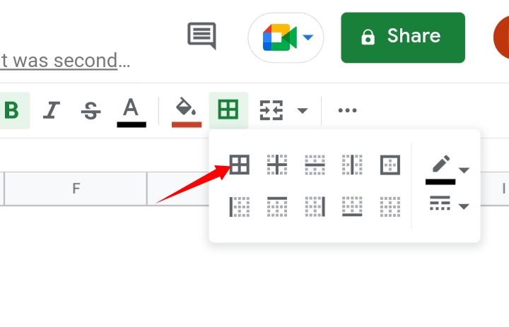
The border-style is added to the hidden cells. This would show the gridlines of the selected cell range or the entire worksheet.
Final Thoughts.
This is an important tool for highlighting and separating important parts of the data set for better viewing and analysis. Now you know How To Hide And Show Gridlines In Google Sheets. I hope you found this review helpful. Thanks for reading.


