Google Sheets have a lot of features used to aid several aspects of data entry easily. Due to its versatility, functions and formulas used are prone to potential errors which implies that Google sheets are not a perfect tool and can also make mistakes.
When errors occur, they are not indicated by the operating system which makes them difficult to understand and resolve. Amongst these errors, the circular dependency error is one of the most common forms that can be displayed on your worksheet, if not careful.
In this tutorial, we are going to discuss what this error means, the causes and how they can be fixed.
How to Fix ‘Circular Dependency Detected’ Error in Google Sheets
This error occurs when the formula used, exists in the range where the calculation takes place which means the input is directly in combination with the formula.
This generates an error where the formula needs to produce results whereby the input becomes the output of the formula and seizes the formula operations entirely.
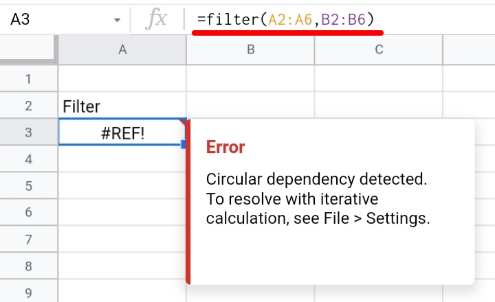
When the error occurs, the error would become highlighted in red, and the text entered previously would change to #REF!.
Click on the highlighted cell, a notification is displayed stating:
“Circular Dependency detected. To resolve with iterative calculation. See File>Spreadsheet settings”.
We can resolve the error message by changing the format of the formula or the parameters stated in the worksheet.
This error can occur under three circumstances.
- The formula is inside the range that you are referring to.
- The formula’s input depends on the output.
- Forgetting the Tab name when using Data from another tab.
We are going to explain and discuss how to solve the circular dependency error and how to spot the cause of the error.
Check out How to Fix Formula Parse Error in Google Sheets.
Problem One: Formula Being inside the Range that is being referred.
This occurs when the cell ranges are wrongly inputted in a formula. A common function that is subject to this error is the SUM function. For instance, we want to add the total sales made daily on each item in column A.
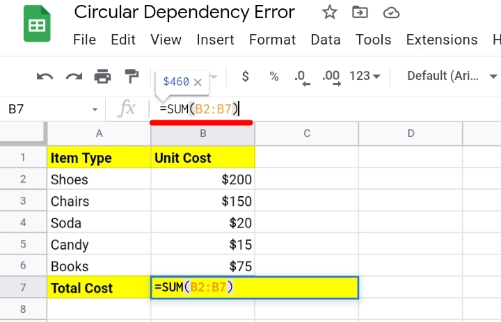
The sales data is listed in cell B2 to cell B6. But below, the error detected is because the cell range stated is B2 to B7 and B7 is the cell that contains the formula. This is the primary cause of the detected circular dependency error.
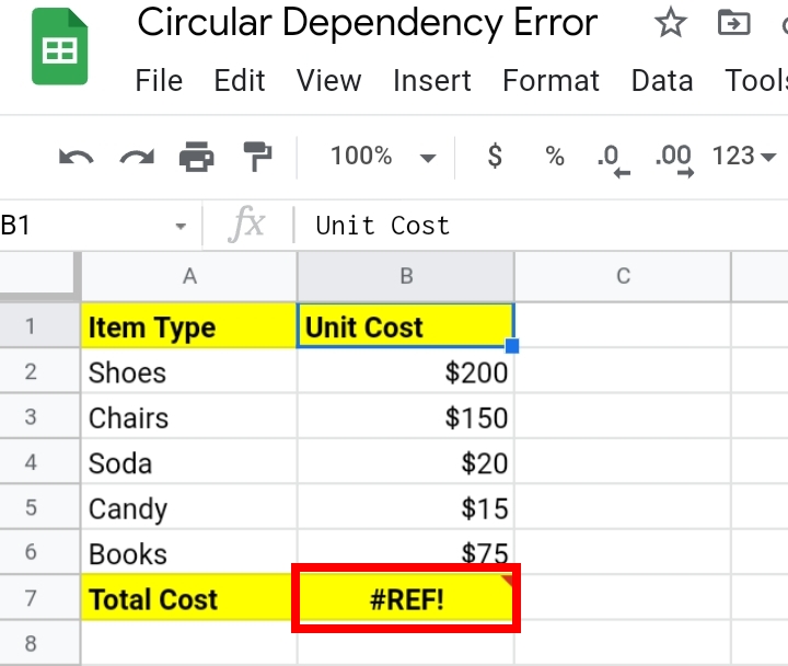
Solution:
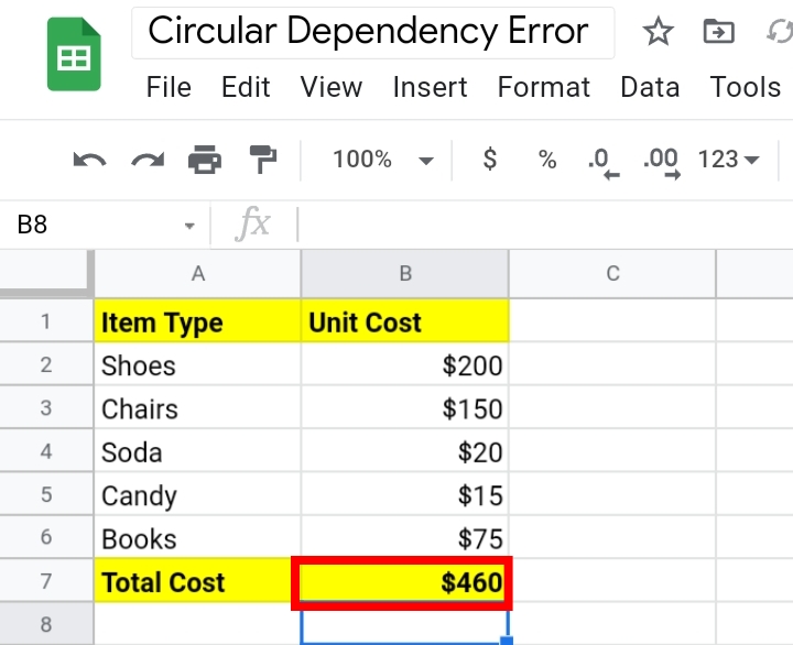
Change the cell range to the correct cell range excluding the result cell, B7. The correct range is inputted as B2:B6. Click Enter and the accurate total of the sales is displayed.
Problem Two: The Formula’s Input depends on the Output.
This error occurs when there are two or more formulas calculating values in the worksheet. These formulas mostly rely on each other.
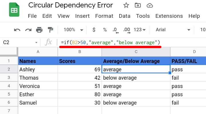
For instance, we have a list of names of some students and their grades in the previous mathematics examination. We want to use the IF function to determine if their grade is higher or lower than the average limit to indicate whether they pass or fail.
=IF(B2>,” Average”, “below average”)
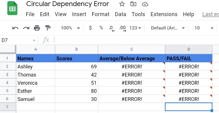
In the sample worksheet below, the cells C2 to C6 and cells D2 to D6 have errors. The cells in column D depend on the output of the results produced in cells in column C.
When the formula contains an error, the other formulas on the worksheet automatically receive an error because they are dependent on each other.
Solution:
To resolve this error, we have to confirm the formula inputted in column C produces accurate results that won’t affect the formula in column D.
The major cause of the error is that we omitted a condition for the IF function to abide by in the first formula. The correct formula is:
=IF(B2>50, ” Average”, “below average”)
Click enter. The scores above the specified criteria are displayed as Average while the score below, are displayed as below average.
Due to the accurate formula in column C, the results in column D are also valid.
Problem Three: Forgetting Tab Name when using Data from Another Tab.
This occurs when you forget to add the tab name as a reference in the formula. A different tab is where the results of the calculated data of the original sheet are pasted to.
For example, we would use the FILTER function to filter the names of the students whose grades were above 50 marks. Here, the tab name of the first sheet is omitted which makes the circular dependency error pop up.
=FILTER(A2:A6, B2:B6)
Solution:
Indicate the forgotten sheet’s name into the formula, by adding its tab name, to describe which tab the worksheet is located.
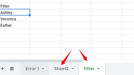
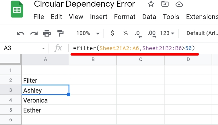
The correct formula is:
=FILTER(Sheet2!A2:A6, Sheet2!B2:B6 >50)
Click Enter. The names of the students are filtered correctly without errors.
Final Thoughts:
Many other errors can appear in your dataset if you are not careful and attentive to the components and positions of the parameters of your formula.
With the highlighted solutions to the problems posed by the circular dependency error. I hope you found this article helpful. Thanks for reading.


