It is a very common thing when working with Google Sheets that you see a set of data with first and last names listed in two different columns.
Having these data stored in two separate columns can help analyze data more efficiently. However, sometimes you may need to combine these columns; the first name and the last name.
In this article, we will learn six ways to combine first and last names in Google Sheets.
So, let’s get started.
Using the Ampersand Operator
This is the simplest and the easiest way to combine the first and last names. The Ampersand (&) is used to combine multiple together, regardless of their data types.
1. Choose the empty cell adjacent to the cells you wish to combine its first and last name.
2. Type in it the following formula, = A2 & B2
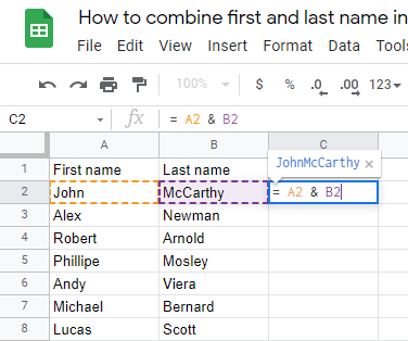
This will print out the last name in only one cell, so how to write it out in all cells in one go? We have two ways:
- You can simply copy and paste the formula in every cell, changing the numbers for sure.
- Click and drag the left square on the lower right corner of the cell to all the cells, as shown.
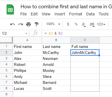
3. You will now have all the first and last names printed in the full name row, as shown.
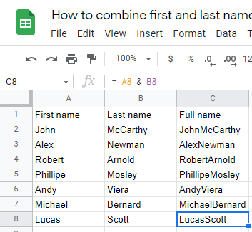
But the names don’t appear to be right without having a space between the first and last name, so how to add a space between them?
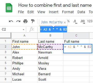
The answer is by having two ampersands and a space in between. Just type the following formula,
= A2 & ” ” & B2
Using the CONCAT Function
The Concat function allows you to combine two values of an argument with this formula, =CONCAT ( value1, value2 )
Where value1 is the first name and value2 is the last name, so the formula will be the following, = CONCAT ( A2, B2 )
So, the steps will be the following:
1. Choose the empty cell adjacent to the cells you wish to combine its first and last name.
2. Type in it the following formula, = CONCAT ( A2, B2 )
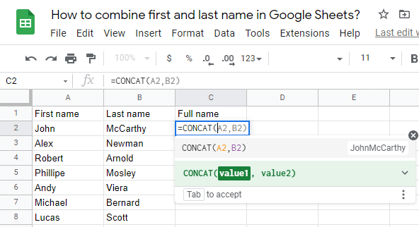
3. As shown, you will now have the full name printed in the cell (C2) but without spacings.
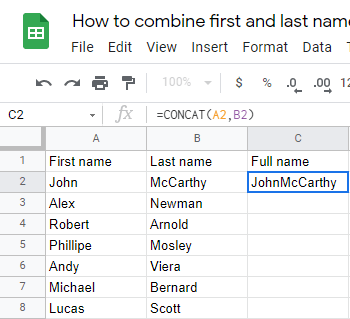
You can print the full name of all rows with the same steps as we did by using the Ampersand operator by either copying and pasting the formula in every cell or by dragging the blue square in the lower right corner of the cell.
The problem with using the CONCAT function is that you can’t add a space between the combined words because, as we said, it only takes two values in the argument.
Using the CONCATENATE Function
This is the best way to combine the first and last names with the formula, =CONCATENATE (string1, [string2, …])
The most significant advantage of using the CONCATENATE function is that it allows you to combine any number of values, easily adding a space between names with the strings simply separated by a comma.
1. Choose the empty cell adjacent to the cells you wish to combine its first and last name.
2. Type in it the following formula, = CONCATENATE ( A2, B2 )
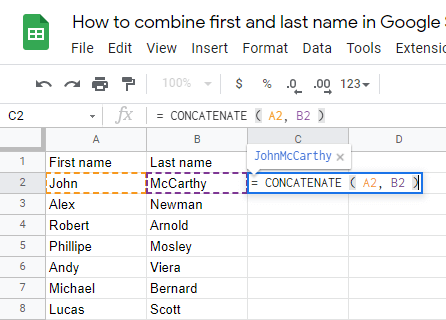
3. As shown, you will now have the full name printed in the cell (C2) but without spacings.
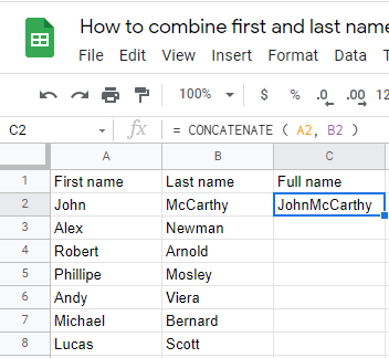
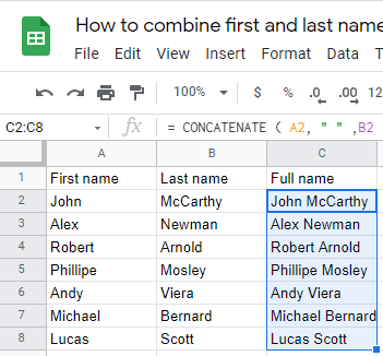
As we said, it’s easy to add a space in the CONCATENATE function by only adding a double quote with a space between the two strings. Just type the following formula, = CONCATENATE ( A2, ” “, B2 )
You can also print the full name of all rows with the same steps as we said earlier by copying and pasting the formula in every cell or by dragging the blue square in the lower right corner of the cell.
Using the TEXTJOIN Function
The TEXTJOIN function combines two or more text values of an argument together, with the formula as follows,
TEXTJOIN ( delimiter, ignore_empty, text1, [text2, …] )
It’s composed of:
- delimiter: This is a necessary argument that specifies the system’s delimiter to separate the text after it has been concatenated. Users prefer to use white space as a delimiter most of the time. You may, however, use any other special characters you want.
- ignore_empty: It’s also a required argument that accepts two logical inputs, TRUE or FALSE, to indicate whether or not the formula should disregard empty cells. If TRUE is used, the formula will disregard any empty cells or values in the calculation.
- Text1 & text2 are just the range of cells you want to combine.
So, the steps will be the following:
1. Choose the empty cell adjacent to the cells you wish to combine its first and last name.
2. Type in it the following formula,
= TEXTJOIN (” “, TRUE, A2, B2 )
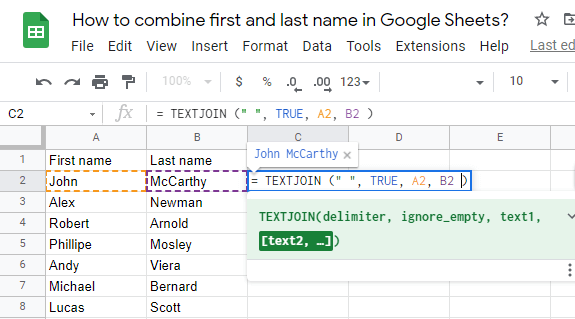
3. As shown, you will now have the full name printed in the cell (C2) but with spacings between words.
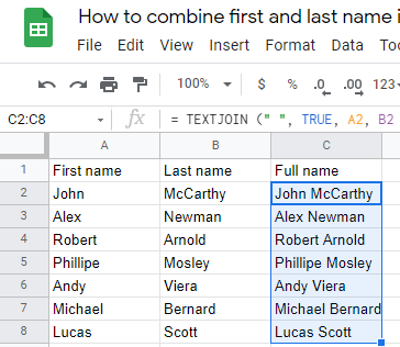
You can also print the full name of all rows with the same steps as we said earlier by copying and pasting the formula in every cell or by dragging the blue square in the lower right corner of the cell.
Note: When using the TEXTJOIN function to concatenate first and last names, you can try various special characters as a delimiter, as in this formula.
=TEXTJOIN(“_”, TRUE, A2, B2)
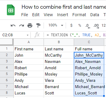
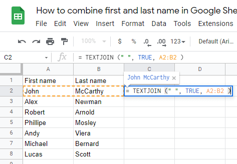
There is a better technique of combining neighboring cells using the TEXTJOIN function. You can use the last parameter to refer to a specific range, and it will combine all of the cells in that range.
To link the first and last names in A2 and B2, you simply need to mention the range A2:B2 in the formula. = TEXTJOIN ( ” “, TRUE, A2:B2 )
Using the Smart Fill Option
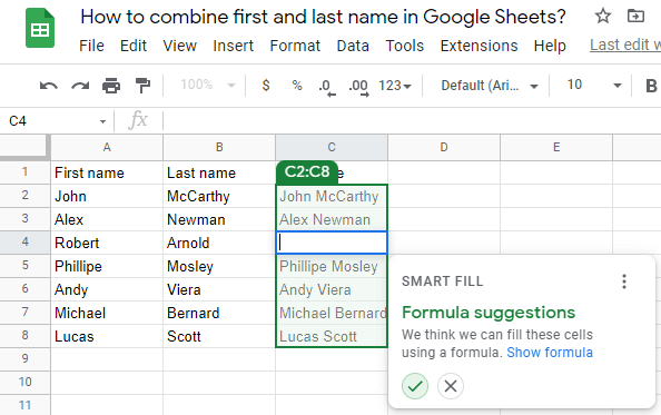
Smart Fill is an AI-generated option that is very popular among Google Sheets users. It can generate formulas as it understands your data entry patterns then recommends a proper option to complete it by either offering a formula or auto-completing the remaining cells.
The steps to use this option are very easy.
All you need to do is type the first and last names combined manually in the full name cells (C2) and (C3). Then, a pop up will appear, with Google Sheets suggesting a formula to autofill the remaining cells in the same pattern shown below.
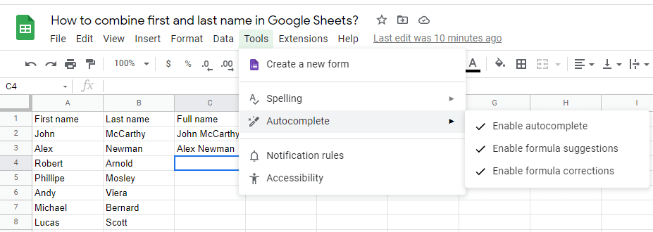
If the Smart Fill option is not working with you, you can enable it manually by doing the following steps:
1. Click on Tools from the tool menu above.
2. Choose Autocomplete.
3. You will see three options, Enable autocomplete, Enable formula suggestions and Enable formula corrections. We suggest that you enable all three options.
Note: You can use the shortcut to enable the Smart Fill option,
CTRL + SHIFT + Y
Using the Apps Script
The Google Apps Script framework should be for you if you want to automate tasks rather than manually inputting equations and establishing ranges.
1. Click on Extensions from the tool menu above.
2. Choose Apps Script.
3. Copy and paste the following code there.
function ConCat() {
var sheet = SpreadsheetApp.getActiveSpreadsheet().getSheetByName(“Data”);
var lastRow = sheet.getLastRow();
//Get values from the First Name column
var firstName = sheet.getRange(2, 1, lastRow,1).getValues();
//Get values from the Last Name column
var lastName = sheet.getRange(2, 2, lastRow,1).getValues();
//Create an empty array that can hold the concatenated values
var fullName = [];
//Add items to the fullName array
for(var i=0; i<lastRow; i++){
fullName[i] = [firstName[i][0]+” “+lastName[i][0]]
}
//Post the result back to Full Name column (column C) starting from row 2
sheet.getRange(2, 3, lastRow, 1).setValues(fullName);
}
4. Go to the Apps Script menu, select Run, and you’ll see the result that automatically combines the first and last names, then populates column C with the combined output.
Conclusion
In this tutorial, you have learned six ways to combine first and last names in Google Sheets.
What are you waiting for? Open up your Google Sheets document, choose one of the six ways and combine names.


